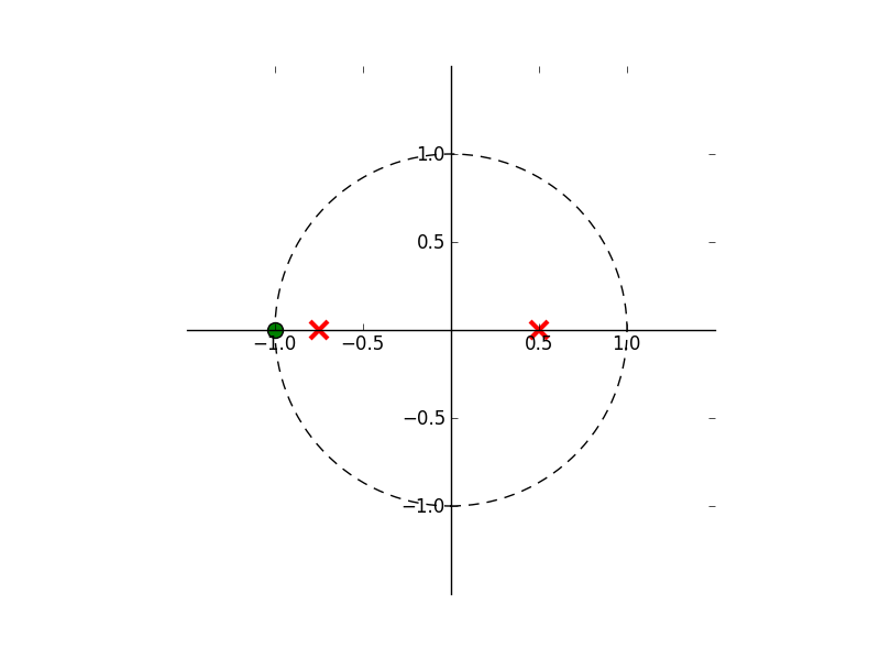
Python zplane function

Python is a popular general purpose programming language with powerful numerical and scientific packages, numpy and scipy.  The Python ecosystem also has a impressive plotting package, matplotlib.  The language and packages (the Python ecosystem) creates an ideal computing platform for Science and Engineering analysis and design. 

But the current distributions does not include a zplane function which many DSP'ers might use because it is availabe in other packages Matlab, Octave, etc.  Below is a function to implement similar behavior to the common used zplane function.

The zplane function takes the numerator and denominator polynomial representation of a transfer function and plots the complex z-plane poles and zeros.

 

 

For those unfamiliar with a numerical computing package, polynomials are usually represented least order coefficient to the highest order coefficient.  An array assignment might look like the following, where *N* is the polynomial order.

The function below will plot a complex zplane given an array of b and a coefficients, numerator and denominator respectively. 

This code requires the following packages:

• matplotlib (plotting routines)
• numpy  (array object and roots)

Example usage:

>>> import numpy as np
# If the code is in a file called plot_zplane.py
>>> from plot_zplane import zplane 
>>> b = np.array([0, 1, 1])
>>> a = np.array([1, 1/4., -3/8.])
>>> zplane(b,a)

 

 

Rate this code snippet:
posted by Christopher Felton
Christopher Felton's current favorite projects are implementing DSP digital circuits with MyHDL for FPGAs. More information @ LinkedIn.
Follow @FeltonChris

Works fine, thank you!

I created a little longer example showing also the impulse response and frequency response of the system. For more details see: http://scipy-central.org/item/52/1/zplane-function

I hope your code finds its way to the official scipy.signal distribution.

Thanks for the additional examples!

I don't know if a function like this would be added to the scipy package.  Functions that rely on plotting are hard to fit into packages like scipy.  A more appropriate spot might be the matplotlib.mlab package.  Which isn't a perfect fit either since the z-plane and s-plane are specific to signal processing.