DFT Graphical Interpretation: Centroids of Weighted Roots of Unity

• Basics
• DFT_FFT
• Tutorials

Introduction

This is an article to hopefully give a better understanding to the Discrete Fourier Transform (DFT) by framing it in a graphical interpretation. The bin calculation formula is shown to be the equivalent of finding the center of mass, or centroid, of a set of points. Various examples are graphed to illustrate the well known properties of DFT bin values. This treatment will only consider real valued signals. Complex valued signals can be analyzed in a similar manner with the only distinction being rotation as well as rescaling will occur. Most of the signals analyzed will be simple pure tones.

Geometric Series Summation Formula

Check out the following factorization pattern:

$$ 1 - x^2 = (1 - x)(1 + x ) $$ $$ 1 - x^3 = (1 - x)(1 + x + x^2 ) $$ $$ 1 - x^4 = (1 - x)(1 + x + x^2 + x^3 ) $$ $$ 1 - x^5 = (1 - x)(1 + x + x^2 + x^3 + x^4 ) $$ $$ 1 - x^6 = (1 - x)(1 + x + x^2 + x^3 + x^4 + x^5 ) $$ $$ 1 - x^7 = (1 - x)(1 + x + x^2 + x^3 + x^4 + x^5 + x^6 ) $$

It can be generalized using summation notation:

$$ 1 - x^N = (1 - x) \sum_{n=0}^{N-1} {x^n} $$

As long as $ x \neq 1 $ both sides can be divided by $ (1 - x) $ and the equation reversed to yield:

$$ \sum_{n=0}^{N-1} {x^n} = { { 1 - x^N } \over { 1 - x } } $$

The expression represented by the summation is called a geometric series and the equation is known as the Geometric Series Summation Formula. It will be used in the future so knowing how it is derived is useful.

The Discrete Fourier Transform

Suppose there is a signal represented by a sequence of $ N $ values $ S_n $, where $ n $ ranges from $ 0 $ to $ N-1 $.

This is the mathematical summation definition of the DFT of the signal according to common convention:

$$ Z_k = { 1 \over N } \sum_{n=0}^{N-1} { S_n e^{ -i2 \pi { k \over N } n } } $$

The leading $ 1/N $ value is called a normalization factor. Some conventions have a normalization factor of 1, others use $ 1/\sqrt{N} $. There are reasons for each. For this article, $ 1/N $ is the correct one.

The negative sign in the exponent is also by convention. This article will use it because it is more of a common convention than not having it. The mathematics of the two alternatives are equivalent.

The formula can be greatly simplified in appearance and understanding by making a substitution.

$$ R_k = e^{ -i2 \pi { k \over N } } $$

Each $ R_k $ is an Nth Root of Unity. This is easily proved:

$$ R_k^N = (e^{ -i2 \pi { k \over N } })^N = e^{ -i2 \pi k } = (e^{ -i2 \pi })^k = 1^k = 1 $$

Substituting the definition of $ R_k $ into the definition of the DFT gives a simpler version.

$$ Z_k = { 1 \over N } \sum_{n=0}^{N-1} { S_n R_k^n } $$

The DFT definition is now recognizable as a straight up average formula: Add up N items, divide by N, and you get the average. 

Since the items are complex numbers, they correspond to points on the complex plane. Therefore, the average can be viewed as the centroid of the set of points. Each item is an Nth Root of Unity rescaled by the value of the signal. You can think of the Roots of Unity as being spokes on a wheel and the rescaling factor how much the spoke is lengthened or shortened. In the case of a complex signal, the spoke will also be rotated.

DFTs of Constant Signals

The simplest possible non-zero signal is a constant signal where every value is the same.

$$ S_n = v $$

In this case, the constant value can be factored out of every term in the DFT summation definition and it becomes:

$$ Z_k = { 1 \over N } \sum_{n=0}^{N-1} { v R_k^n } = v \cdot { 1 \over N } \sum_{n=0}^{N-1} { R_k^n } $$

The summation formula now becomes a geometric series and the geometric series summation formula can be applied for all values of $ k $, except for $ k = 0 $. This is because $ R_0 = 1 $ which would make the denominator $ 0 $.

$$ Z_k = v \cdot { 1 \over N } \cdot { { 1 - R_k^N } \over { 1 - R_k } } $$

Since $ R_k $ is a $ Nth $ root of unity $ R_k^N = 1 $.  This makes the numerator equal to zero.

$$ Z_k = v \cdot { 1 \over N } \cdot { 0 \over { 1 - R_k } } = 0 $$

The DFT of a constant signal is zero on all bins where $ k > 0 $.

The DC Bin

The first bin, $ Z_0 $, is different than the rest in that the base Root of Unity is one itself ($ R_0 = 1 $). Therefore the summation equation gets greatly simplified.

$$ Z_0 = { 1 \over N } \sum_{n=0}^{N-1} { S_n R_0^n } = { 1 \over N } \sum_{n=0}^{N-1} { S_n } $$

$ Z_0 $ is the simple arithmetic average of the signal values. It is called the "DC bin" from applications where the signal is a voltage level. DC stands for Direct Current. When the DC component is subtracted from the signal, the rest of the signal is zero centered. With a real valued signal, the average will also be real valued so the imaginary part will always be zero.

In the case of a constant signal, like in the previous section, the value of the DC bin is the value of the signal points.

$$ Z_0 = { 1 \over N } \sum_{n=0}^{N-1} { v } = v \cdot { 1 \over N } \sum_{n=0}^{N-1}{ 1 } = v \cdot { 1 \over N } \cdot N = v $$

Skip Sizes

When an Nth Root of Unity is raised to an integer power the result is also an Nth Root of Unity.

$$ R_k^n = (e^{ -i2 \pi { k \over N } })^n = e^{ -i2 \pi { { kn } \over N } } = R_{kn} $$

Inserting this into the DFT definition modifies it slightly:

$$ Z_n = { 1 \over N } \sum_{n=0}^{N-1} { S_n R_{kn} } $$

Unfurling the summation notation for the first six bins shows the pattern more clearly:

$$ Z_0 = { 1 \over N }( S_0 R_0 + S_1 R_0 +S_2 R_0 +S_3 R_0 + ... + S_{N-1} R_0 ) $$ $$ Z_1 = { 1 \over N }( S_0 R_0 + S_1 R_1 +S_2 R_2 +S_3 R_3 + ... + S_{N-1} R_{N-1} ) $$ $$ Z_2 = { 1 \over N }( S_0 R_0 + S_1 R_2 +S_2 R_4 +S_3 R_6 + ... + S_{N-1} R_{N-2} ) $$ $$ Z_3 = { 1 \over N }( S_0 R_0 + S_1 R_3 +S_2 R_6 +S_3 R_9 + ... + S_{N-1} R_{N-3} ) $$ $$ Z_4 = { 1 \over N }( S_0 R_0 + S_1 R_4 +S_2 R_8 +S_3 R_{12} + ... + S_{N-1} R_{N-4} ) $$ $$ Z_5 = { 1 \over N }( S_0 R_0 + S_1 R_5 +S_2 R_{10} +S_3 R_{15} + ... + S_{N-1} R_{N-5} ) $$

What can be seen is the skip size on the set of Roots of Unity for each bin is the same as the index for that bin.  The simplest form for the subscript of the Root of Unity is $ kn $ modulo $ N $.  Since $ R_0 = 1 $, all the references to $ R_0 $ can be removed from the formulas.  They are left intact for the purpose of clarity.

Explanation of the Figures

The figures are drawn by a program custom written just for this blog article. They are designed to show graphically the relationship between the shape of the signal and the resulting point sets which come from the DFT equation. The signal value points are shown on the upper right graph. The horizontal axis spans from 0 to $ 2\pi $ angle wise and is segmented from 0 to $N$. The data points, consisting of one frame, range from 0 to $ N-1 $, never reaching the right vertical axis. The vertical axes range from -1 to 1 and have tic marks every tenth.

The six polar graphs at the bottom show the calculations of the first six bins of the DFT on the complex plane. The set of $ R_k $ points are shown around the circumference of the circle. The horizontal and vertical tic marks show tenths along the radii.  The outer circle is the unit circle.

The blue circle is centered on the centroid location. The first graph is for $ Z_0 $, also known as the DC bin. In the constant signal example shown in Figure 1, all the data values, and thus the centroid, all fall on the same spot. The second polar graph is for $ Z_1 $. The skip size is one, so the function is wrapped once around the circle. The third polar graph is for $ Z_2 $. In a like manner, the skip size is two, so the function is wrapped twice around the circle hitting every other $ R_k $. The last three are for $ Z_3 $, $ Z_4 $, $ Z_5 $, with skip sizes of 3, 4, and 5. Of course, these are also the number of times the function is stretched and wrapped around the circle.

The data points, and the tracer lines between them, are colored to fade from green to red. This allows the sequence of points to be seen in the polar graphs. Figure 1 shows the plots of a constant signal at one half. The skip sizes for each polar graph should be determinable by the coloration of the points.

The equation of the generated signal is given on the top left. The frequency is measured in cycles per frame, or equivalently, cycles per N points.

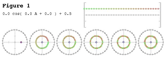
A prime number for $ N (=31) $ was selected so that all the $ R_k $ points were hit no matter what the step size.

Integer Frequency Signals

The first set of figures show the DFT calculations for the first five integer frequencies on the six bins.

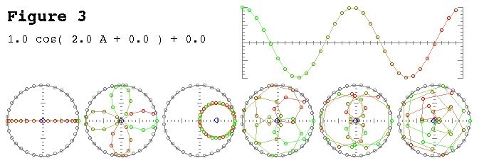
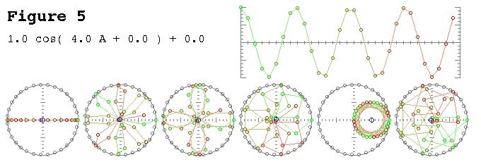
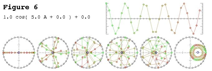
There are four main take aways from this set of figures. First, the DC bin is zero because a tone signal with a whole number of cycles will be centered on the zero line. Second, when the number of cycles matches the number of wrappings, all the bumps line up and the centroid is off center. Third, when the number of cycles doesn't match the number of wrappings, the bumps are radially distributed, and by symmetry the centroid is on center. Fourth, the magnitude of the centroid in the matching case is half the amplitude of the signal, just as the center of a circle is at half the diameter.

Non-Integer Frequency Signals

This next set of figures shows samples with non-integer frequencies.

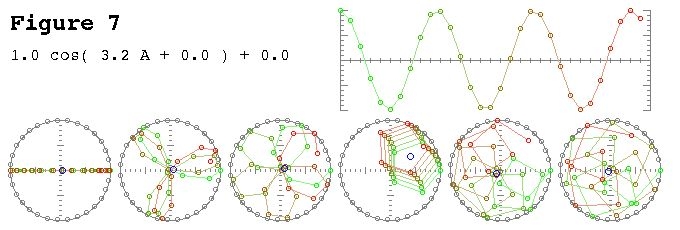
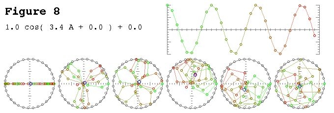
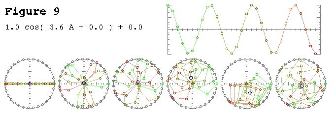
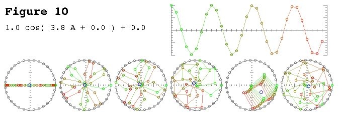
Since there is not a set of whole cycles, and the signal starts at an extreme, the average value is no longer zero so the DC bin is no longer centered. Also, the partial cycle throws off the radial symmetry so the all the bins are non-zero. The most off center results occur where the bin wrapping counts are closest to the frequency and taper off from there. The centroid switches sides on the two bins with the wrapping counts on either side of the fractional frequency.

Here is the halfway point.

Notice that $ Z_3 $ and $ Z_4 $ are nearly opposite each other.

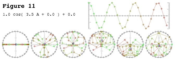
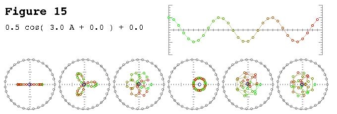
Varying the Phase

This set of figures show what happens as you adjust the phase value.

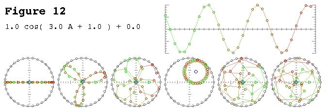
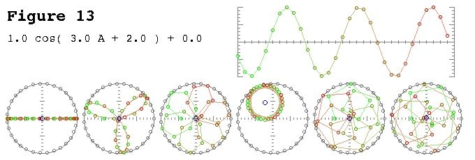
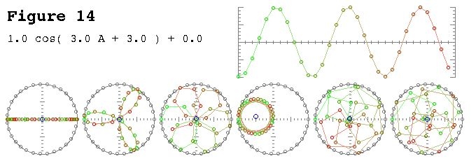
The phase shift translates into a rotation. The amount of the rotation is dependent on the bin number. For integer frequencies, the rotation in the corresponding bin will equal the phase shift.

Varying the Magnitude

Varying the magnitude is the easiest to understand.

Any rescaling of the signal gets factored out of the summation and applies to the sum as a whole. Therefore the polar graphs and centroids are resized by the same factor.

Signals with a DC Offset

This set of figures shows the effect of moving the signal up and down vertically by adding a constant value.

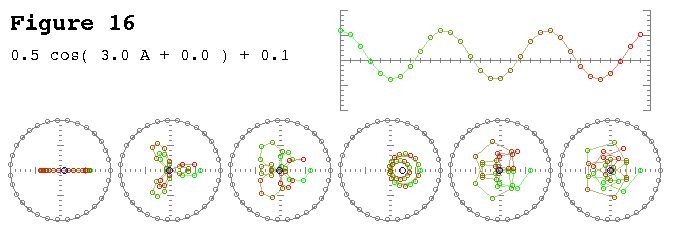
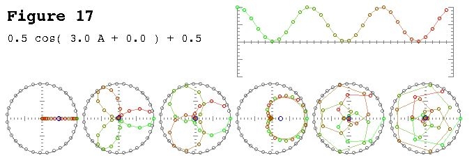
This changes the shapes of the polar graphs slightly, but does not have any effects on the location of the centroids, except in the DC bin.

$$ Z_k = { 1 \over N } \sum_{n=0}^{N-1} { ( S_n + d ) R_k^n } = { 1 \over N } \sum_{n=0}^{N-1} { S_n R_k^n} + { 1 \over N } \sum_{n=0}^{N-1} { d R_k^n} = { 1 \over N } \sum_{n=0}^{N-1} { S_n R_k^n } + 0 $$

The Sum of Two Signals

The centroid of a sum is the sum of centroids. Mathematically it is said like this:

$$ Z_k = { 1 \over N } \sum_{n=0}^{N-1} { ( S_n + T_n ) R_k^n } = { 1 \over N } \sum_{n=0}^{N-1} { S_n R_k^n } + { 1 \over N } \sum_{n=0}^{N-1} { T_n R_k^n } $$

Where $ S_n $ and $ T_n $ are the two signals. In the case of two distinct integer value frequency signals, the results of the DFT will be completely separable. The two bin values associated with the two frequencies will be the only off center ones.

Here is a sample:

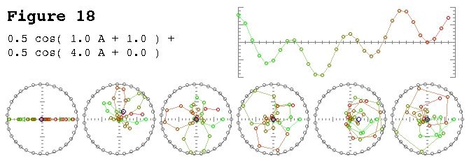
The only bins that are off center are $ Z_1 $ and $ Z_4 $. The angles also reflect the phase values.

Bin Symmetry of Real Signals

For real valued signals the top half of the DFT bin set will be the complex conjugate of the bottom half. In terms of the polar graphs, this can be understood by recognizing that it is the equivalent centroid calculations with the signal being wrapped counter-clockwise instead of clockwise. The result is the mirror image reflected by the real axis. This is exactly what complex conjugates are.

$$ R_p = \overline{ R_{N-p} } $$

$$ R_p^2 = R_{2p} = \overline{ R_{N-p}^2 } = \overline{ R_{2N-2p} } = \overline{ R_N } \cdot \overline{ R_{N-2p} } = 1 \cdot \overline{ R_{N-2p} } = \overline{ R_{N-2p} } $$

This same pattern occurs with the higher powers of $ R_p $.  This shows that the powers work in reverse just as well as forward.

The Nyquist Bin

When $ N $ is an even number, the $ N/2 $ bin is known as the Nyquist bin. The only Roots of Unity used in the centroid calculation will be $ R_0 $ and $ R_{N/2} $, also known as 1 and -1. If the signal consists of only real values, then the resulting centroid will be real and the imaginary part will be zero. Another way to convince yourself of this is in the real signal case, the Nyquist bin has to equal its own conjugate.

Conclusion

DFT bin values can be seen as the centroids of polar graphed signal points on the complex plane. In this manner the well known properties of DFTs can be visualized qualitatively. Although this article only dealt with simple pure tone samples, the ideas can be extended to more complicated signals and even complex signals. An understanding of the principles outlined should help in knowing the strengths and weaknesses of DFT analysis in particular circumstances.

[Edit 2015-06-01: Swap n and k in subscripts]

Sign in