


Model a Sigma-Delta DAC Plus RC Filter
Sigma-delta digital-to-analog converters (SD DAC’s) are often used for discrete-time signals with sample rate much higher than their bandwidth. For the simplest case, the DAC output is a single bit, so the only interface hardware required is a standard digital output buffer. Because of the high sample rate relative to signal bandwidth, a very simple DAC reconstruction filter suffices, often just a one-pole RC lowpass. In this article, I present a simple Matlab function that models the combination of a basic SD DAC and one-pole RC filter. This model allows easy evaluation of the overall performance for a given input signal and choice of sample rate, R, and C.

DAC Zero-Order Hold Models
This article provides two simple time-domain models of a DAC’s zero-order hold. These models will allow us to find time and frequency domain approximations of DAC outputs, and simulate analog filtering of those outputs. Developing the models is also a good way to learn about the DAC ZOH function.

Decimators Using Cascaded Multiplierless Half-band Filters
In my last post, I provided coefficients for several multiplierless half-band FIR filters. In the comment section, Rick Lyons mentioned that such filters would be useful in a multi-stage decimator. For such an application, any subsequent multipliers save on resources, since they operate at a fraction of the maximum sample frequency. We’ll examine the frequency response and aliasing of a multiplierless decimate-by-8 cascade in this article, and we’ll also discuss an interpolator cascade using the same half-band filters.

Pentagon Construction Using Complex Numbers
A method for constructing a pentagon using a straight edge and a ruler is deduced from the complex values of the Fifth Roots of Unity. Analytic values for the points are also derived.

Multiplierless Half-band Filters and Hilbert Transformers
This article provides coefficients of multiplierless Finite Impulse Response 7-tap, 11-tap, and 15-tap half-band filters and Hilbert Transformers. Since Hilbert transformer coefficients are simply related to half-band coefficients, multiplierless Hilbert transformers are easily derived from multiplierless half-bands.


Interpolator Design: Get the Stopbands Right
In this article, I present a simple approach for designing interpolators that takes the guesswork out of determining the stopbands.


Return of the Delta-Sigma Modulators, Part 1: Modulation
About a decade ago, I wrote two articles: Modulation Alternatives for the Software Engineer (November 2011) Isolated Sigma-Delta Modulators, Rah Rah Rah! (April 2013) Each of these are about delta-sigma modulation, but they’re...

Simple Discrete-Time Modeling of Lossy LC Filters
There are many software applications that allow modeling LC filters in the frequency domain. But sometimes it is useful to have a time domain model, such as when you need to analyze a mixed analog and DSP system. For example, the...
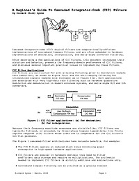
A Beginner's Guide To Cascaded Integrator-Comb (CIC) Filters
This article discusses the behavior, mathematics, and implementation of cascaded integrator-comb filters.

Minimum Shift Keying (MSK) - A Tutorial
Minimum Shift Keying (MSK) is one of the most spectrally efficient modulation schemes available. Due to its constant envelope, it is resilient to non-linear distortion and was therefore chosen as the modulation technique for the GSM cell phone...
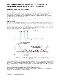
FFT Interpolation Based on FFT Samples: A Detective Story With a Surprise Ending
This blog presents several interesting things I recently learned regarding the estimation of a spectral value located at a frequency lying between previously computed FFT spectral samples. My curiosity about this FFT interpolation process was triggered by reading a spectrum analysis paper written by three astronomers.

Two Easy Ways To Test Multistage CIC Decimation Filters
This article presents two very easy ways to test the performance of multistage cascaded integrator-comb (CIC) decimation filters. Anyone implementing CIC filters should take note of the following proposed CIC filter test methods.

Understanding and Relating Eb/No, SNR, and other Power Efficiency Metrics
Introduction Evaluating the performance of communication systems, and wireless systems in particular, usually involves quantifying some performance metric as a function of Signal-to-Noise-Ratio (SNR) or some similar measurement. Many systems...

Handling Spectral Inversion in Baseband Processing
The problem of "spectral inversion" comes up fairly frequently in the context of signal processing for communication systems. In short, "spectral inversion" is the reversal of the orientation of the signal bandwidth with...

An Interesting Fourier Transform - 1/f Noise
Power law functions are common in science and engineering. A surprising property is that the Fourier transform of a power law is also a power law. But this is only the start- there are many interesting features that soon become apparent. This may...

A Fixed-Point Introduction by Example
Introduction The finite-word representation of fractional numbers is known as fixed-point. Fixed-point is an interpretation of a 2's compliment number usually signed but not limited to sign representation. It...

Understanding and Implementing the Sliding DFT
Introduction In many applications the detection or processing of signals in the frequency domain offers an advantage over performing the same task in the time-domain. Sometimes the advantage is just a simpler or more conceptually...

Polyphase Filters and Filterbanks
ALONG CAME POLY Polyphase filtering is a computationally efficient structure for applying resampling and filtering to a signal. Most digital filters can be applied in a polyphase format, and it is also possible to create efficient resampling...


