Two Bin Exact Frequency Formulas for a Pure Real Tone in a DFT
Introduction
This is an article to hopefully give a better understanding of the Discrete Fourier Transform (DFT) by deriving exact formulas for the frequency of a real tone in a DFT. This time it is a two bin version. The approach taken is a vector based one similar to the approach used in "Three Bin Exact Frequency Formulas for a Pure Complex Tone in a DFT"[1]. The real valued formula presented in this article actually preceded, and was the basis for the complex three bin case.
Once again, the emphasis on exactness has to do with mathematical correctness and theoretical understanding, not necessarily superior performance in a practical application. However, in the two bin case I know of no approximation formulas that are computationally simpler and/or more robust. The first exact two bin real tone formula I am aware of was presented by Martin Vicanek[2]. He made the observation that the two bin case is actually overdetermined and should be solvable. Shortly after that I derived one that was based on the approach I took with my original three bin version [3]. Being exact, it worked fine in the noiseless case, but performed poorly compared to Vicanek's in the presence of noise. Consequently I have not published it.
In response to another comp.dsp thread earlier this year in which Michael Plet presented another two bin formula [4], I revisited the topic and derived the approach presented in this article. The first version was comparable to Vicanek's, but slightly worse. An adjustment made to the formula made it slightly better. All three are significantly better than my original attempt.
A Pure Real Tone Sequence
This is the same real pure tone formula I use in all the blog articles. The frequency term ($\alpha$) is expressed in units of radians per sample which makes the formula as simple as possible. $$ S_n = M \cos( \alpha n + \phi ) \tag {1} $$ The frequency in the formula can readily be converted from units of cycles per frame using this formula: $$ \alpha = f \cdot \frac{ 2\pi }{ N } \tag {2} $$ The frequency in Hz (cycles per second) depends on the duration of the sampling frame.
The Discrete Fourier Transform
This is a formula for a bin value of the Discrete Fourier Transform (DFT) for any signal. $$ Z_k = \frac{ 1 }{ N } \sum_{n=0}^{N-1} { S_n e^{ -i\beta_k n } } \tag {3} $$ Similar to the signal definition, the "frequency term" is the bin index in terms of cycles per frame which can be translated into a unit of radians per sample to simplify the DFT definition. $$ \beta_k = k \cdot \frac{ 2\pi }{ N } \tag {4} $$
Pure Real Tone Bin Value Formula
The bin value of a pure real tone can be found without the need to do a summation by plugging (1) into (3) and applying the formula for a summation of a geometric series. The result is the the following formula: $$ Z_k = \frac{ M }{ 2N } \left[ \frac{ U e^{ i\beta_k } - V } { \cos( \alpha ) - \cos( \beta_k ) } \right] \tag {5} $$ Where: $$ U = \cos( \alpha N + \phi ) - \cos(\phi) \tag {6} $$ $$ V = \cos( \alpha N -\alpha + \phi ) - \cos( -\alpha + \phi ) \tag {7} $$ The derivation can be found in my blog article appropriately titled "DFT Bin Value Formulas for Pure Real Tones" [5]. Please note that the formula has a pluggable discontinuity at integer frequencies in terms of cycles per frame. Fortunately, this discontinuity is rendered irrelevant in the frequency formula.
Separating into Real and Imaginary Parts
The bin value, which is a complex value, can be expressed in Cartesian form with two real values. $$ Z_k = x_k + i \cdot y_k \tag {8} $$ Euler's equation is required in order to separate (5) into its real and imaginary components. An intuitive understanding of this magnificent equation is presented in my first blog article[6]. $$ e^{ i\beta_k } = \cos( \beta_k ) + i \cdot \sin( \beta_k ) \tag {9} $$ The two separate real valued equations for a single bin look like this: $$ x_k = \frac{ M }{ 2N } \left[ \frac{ U \cos( \beta_k ) - V } { \cos( \alpha ) - \cos( \beta_k ) } \right] \tag {10} $$ $$ y_k = \frac{ M }{ 2N } \left[ \frac{ U \sin( \beta_k ) } { \cos( \alpha ) - \cos( \beta_k ) } \right] \tag {11} $$
A System of Equations Using Another Bin
The last two equations, (10) and (11), can be cross multiplied to produce these two equations for bin $k$: $$ \cos( \alpha ) \cdot x_k - \cos( \beta_k ) \cdot x_k = \frac{ M }{ 2N } \left[ U \cos( \beta_k ) - V \right] \tag {12} $$ $$ \cos( \alpha ) \cdot y_k - \cos( \beta_k ) \cdot y_k = \frac{ M }{ 2N } U \sin( \beta_k ) \tag {13} $$ These can also be replicated for another bin $j$: $$ \cos( \alpha ) \cdot x_j - \cos( \beta_j ) \cdot x_j = \frac{ M }{ 2N } \left[ U \cos( \beta_j ) - V \right] \tag {14} $$ $$ \cos( \alpha ) \cdot y_j - \cos( \beta_j ) \cdot y_j = \frac{ M }{ 2N } U \sin( \beta_j ) \tag {15} $$ Finally, the unkown value $V$ can be eliminated by subtracting (14) from (12). $$ \cos( \alpha ) \cdot ( x_k - x_j ) - \left[ \cos( \beta_k ) \cdot x_k - \cos( \beta_j ) \cdot x_j \right] = \frac{ M }{ 2N } U \left[ \cos( \beta_k ) - \cos( \beta_j ) \right] \tag {16} $$
A System of Equations In Vector Form
The three equations (16), (13), and (15) can be put into vector form which looks like this: $$ \cos( \alpha ) \cdot \vec A - \vec B = \frac{ M U }{ 2 N } \vec C \tag {17} $$ Where the three vectors are: $$ \vec A = \begin{bmatrix} ( x_k - x_j ) / \sqrt{2} \\ y_k \\ y_j \end{bmatrix} \tag {18} $$ $$ \vec B = \begin{bmatrix} [ \cos( \beta_k ) \cdot x_k - \cos( \beta_j ) \cdot x_j ] / \sqrt{2} \\ \cos( \beta_k ) \cdot y_k \\ \cos( \beta_j ) \cdot y_j \end{bmatrix} \tag {19} $$ $$ \vec C = \begin{bmatrix} [ \cos( \beta_k ) - \cos( \beta_j ) ] / \sqrt{2} \\ \sin( \beta_k ) \\ \sin( \beta_j ) \end{bmatrix} \tag {20} $$ Notice that (16) has been divided by $\sqrt{2}$. The purpose of this adjustment is to make the variance of the difference of the random variables have the same value as the variance of a single variable.
Solving for the Frequency Term
There are many solutions to (17). Suppose that vector $\vec K$ orthogonal to $\vec C$. $$ \vec K \cdot \vec C = 0 \tag {21} $$ As long as $\vec K$ is not orthogonal to $\vec A$ or $\vec B$, then a solution can be easily found by dotting (17) by $\vec K$. $$ \cos( \alpha ) \vec K \cdot \vec A - \vec K \cdot \vec B = 0 \tag {22} $$ Since the right hand side of (17) gets zeroed out, the values of $M$ and $U$ are eliminated, leaving $\alpha$ as the only unknown. $$ \cos( \alpha ) = \frac{ \vec K \cdot \vec B }{ \vec K \cdot \vec A } \tag {23} $$ Once the cosine of the frequency term is found, the actual frequency in cycles per frame can also be found.
Notice that since it is in the numerator and the denominator as a linear factor, the length of $\vec K$ is irrelevant. All that matters is its direction. Since it is constrained to lay within a plane it has one degree of freedom. $$ f = \alpha \cdot \frac{ N }{ 2\pi } = \cos^{-1} \left( \frac{ \vec K \cdot \vec B }{ \vec K \cdot \vec A } \right) \cdot \frac{ N }{ 2\pi } \tag {24} $$ The value given by this equation is a frequency within the range of the DFT. It is possible that the actual frequency is an alias frequency. That is a frequency that is higher than the Nyquist frequency.
Finding the Best Vector
The values of $\vec A$ and $\vec B$ can conceptually be separated into their true values and an error term resulting from noise in the signal. The assumption is that the noise is white noise and thus the error term is a random Gaussian variable. The assumption, at this point in the calculation, is that the vectors $\vec E_A$ and $\vec E_A$ can point in any direction. The assumption that nothing is known about the error term will be addressed in a later blog article. $$ \cos( \alpha ) = \frac{ \vec K \cdot \left( \vec B + \vec E_B \right) }{ \vec K \cdot \left( \vec A + \vec E_A \right) } \tag {25} $$ $$ \cos( \alpha ) = \frac{ \vec K \cdot \vec B + \vec K \cdot \vec E_B }{ \vec K \cdot \vec A + \vec K \cdot \vec E_A } \tag {26} $$ The amount of the error can't be minimized by the appropriate selection of $\vec K$. However, the amount of signal information can be maximized. This is achieved by making $\vec K$ as close to the direction of $\vec A$ and $\vec B$ as possible. This requires projecting a vector onto the plane normal to $\vec C$ to find $\vec K$. Although either $\vec A$ or $\vec B$ could be used, neither is going to be optimal. The good news is because $\vec A$ and $\vec B$ are nearly collinear, choosing between them, or in between them is not that significant. This is borne out by numerical testing. Therefore a good choice would be an average of the two. Since the length is immaterial, a little bit of computation can be saved by simply using the sum instead. $$ \vec D = \vec A + \vec B \tag {27} $$ To make $\vec K$ lie in the plane normal to $\vec C$, some multiple of $\vec C$ needs to be subtracted away. $$ \vec K = \vec D - w \vec C \tag {28} $$ Finding the multiplier is straightforward. Simply dot $\vec K$ with $\vec C$ knowing the result has to be zero. $$ \vec K \cdot \vec C = \vec D \cdot \vec C - w \vec C\cdot \vec C = 0 \tag {29} $$ Solving for the multiplier is simple algebra. $$ w = \frac{ \vec D \cdot \vec C }{ \vec C\cdot \vec C } \tag {30} $$ This results in a final answer for finding the best vector: $$ \vec K = \vec D - \frac{ \vec D \cdot \vec C }{ \vec C\cdot \vec C } \vec C \tag {31} $$ Dotting this vector by $\vec C$ shows by inspection the result will be zero as required.
Precomputing Values
The components of $\vec C$ are independent of the bin values and only dependent on the bin indexes. The values needed for the computation of (31) can be evaluated ahead of time by reconfiguring the equation like this: $$ \vec K = \vec D - \left( \vec D \cdot \frac{ \vec C }{ \| \vec C \| } \right) \frac{ \vec C }{ \| \vec C \| } = \vec D - ( \vec D \cdot \vec P_{k,j} ) \vec P_{k,j} \tag {32} $$ Where the pre-computed unit vector is defined as: $$ \vec P_{k,j} = \frac{ \vec C }{ \| \vec C \| } = \frac{ \vec C }{ \sqrt{ \vec C\cdot \vec C } } \tag {33} $$ In practical usage the two bins will be adjacent, that is $j=k+1$, so only one dimensional arrays are needed. This is because the bins with the highest signal to noise ratio (SNR) will be next to each other (ignoring the bins above the Nyquist frequency, or $N/2$).
Some Numerical Examples
These tests consist of taking a sweep of frequencies from the low end of a bin to the high end. For each frequency a real tone is generated. The phase is swept from zero to $2\pi$. The formulas are evaluated using the same data sets. The Unadjusted column does not have the $\sqrt{2}$ rescaling of (16).
The numbers that are shown are the average and standard deviation of the distribution of frequency errors. The Target Noise Level is the standard deviation of the added noise. The error levels are shown multiplied by 100 for better presentation.
The sample count is 100
and the run size is 4000

Errors are shown at 100x actual value

Target Noise Level = 0.100

Freq   Original        Vicanek      Unadjusted      Improved
---- -------------  -------------  -------------  -------------
4.0  -0.209 33.879  -0.033  1.448  -0.011  1.508  -0.015  1.434
4.1  -0.171 22.714  -0.010  1.201   0.004  1.250   0.004  1.190
4.2   0.099 18.891  -0.026  1.008  -0.012  1.049  -0.015  1.000
4.3  -0.321 18.962  -0.033  0.917  -0.027  0.944  -0.021  0.913
4.4   0.033 15.539  -0.007  0.808   0.005  0.835   0.003  0.804
4.5  -0.580 27.947  -0.000  0.795   0.002  0.818  -0.000  0.790
4.6  -0.194 18.470  -0.000  0.810  -0.017  0.824  -0.014  0.805
4.7   0.165 21.173  -0.009  0.899  -0.021  0.909  -0.020  0.892
4.8  -0.156 36.277   0.015  1.010  -0.001  1.017   0.000  1.001
4.9  -0.037 20.199   0.015  1.187  -0.007  1.181  -0.004  1.172
Just like the complex case, the two bin formulas do best when the frequency is between two bins. This is due to the frequency formula being in essence the result of a weighted average of the two bin values. When the weighting is most even, the combination of the random variables has the least variance.
Conclusion
A solid formula for the calculation of the frequency of a single pure tone from DFT bin values has been presented. There is no guarantee that it is the optimal one. First because the selection of vector $\vec D$ was somewhat arbitrary. Secondly, no special calculations were made to find out information about the nature of the error terms.
Reference
[1] Dawg, Cedron, Three Bin Exact Frequency Formulas for a Pure Complex Tone in a DFT
[2] Vicanek, Martin, Frequency Estimation from two DFT Bins
[3] Dawg, Cedron, Exact Frequency Formula for a Pure Real Tone in a DFT
[4] Plet, Michael, comp.dsp topic: New frequency estimator from two DFT bins
[5] Dawg, Cedron, DFT Bin Value Formulas for Pure Real Tones
[6] Dawg, Cedron, The Exponential Nature of the Complex Unit Circle
- Comments
- Write a Comment Select to add a comment

Hi. Can you tell us, in your Eq. (2) what are the dimensions of the variables 'f' and 'N'?
Thanks.

'f' is 'cycles per frame'.
'N' is 'samples per frame'.
'$2\pi$' is 'radians per cycle'.
'$\alpha$' is 'radians per sample'.
Therefore (2) in units form is:
$$ radians\:per\:sample = cycles\:per\:frame \cdot \frac{radians\:per\:cycle}{samples\:per\:frame} $$
Ced
Hi.
Ah, ...OK. Thanks.
This is a good place to point out these units are the same for equation (4). To me, this unlocks the true meaning of (3), which is the definition of the DFT. Looking at the exponent, $n$ is the sample index so it has units of samples and $\beta_k$ has units of radians per sample. Therefore their product has units of radians. As you know, Euler's equation translates the distance along the circumference of the unit circle to a complex point value on the plane. The negative sign means the distance is measured clockwise on the circle.
The net result is that the $e^{-i \beta_k n }$ term represents an evenly spaced set of points around the unit circle and the spacing between the points is defined by $\beta_k$. Each point is weighted by the corresponding signal value. The weighted points are then summed and divided by the number of points. Therefore, the DFT is actually a center of mass calculation of a weighted set of points around the unit circle.
The multiplication of the signal value ($S_n$) can either be interpreted as a weighting as I did in the previous paragraph, or as a length multiplier as I did in my second blog article: "DFT Graphical Interpretation: Centroids of Weighted Roots of Unity."
Hello,
This question is kind of off topic for this blog entry, you should post it in the forums section instead. You'll get more answers than just mine.
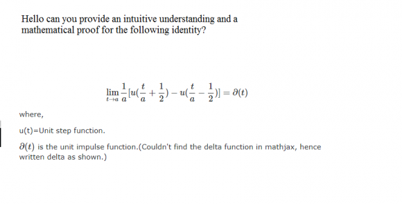
I don't think you have the equation correct, but I do get the gist of it.
The Dirac delta function is zero everywhere except at a certain point where it has the value of infinity. When you integrate over that point the value is one. I think what you are trying to depict is a function that is zero everywhere except a small interval where it is a constant height, the height being defined so that the area of the rectangle that is formed is one. The limit of such a function as the width approaches zero is the Dirac delta function.
Please post any response in the forum. Thanks.
Ced
P.S. Mathjax works within the comment section and the forum.
The equation I think you want is:
$$ \delta(t) = \lim_{a \to 0} \frac{1}{a} \left[ u \left( t + \frac{a}{2} \right) - u \left( t - \frac{a}{2} \right) \right] $$
Ced
Yes sir, you are right, I made a mistake. Sir is there anyway I can notify you if I post my queries in the forum?
I hope I have answered your question though. Notice that the equation I gave is a variation of the definition of a derivative:
$$ f'(x) = \lim_{ \Delta x \to 0 } \frac{ f(x + \Delta x ) - f(x) }{ \Delta x } $$
Loosely speaking, the Dirac Delta function is the derivative of the unit step function and the unit step function is the integral of the Dirac delta function. Since there are infinities involved, a formal mathematical proof is a little more involved and it's been too long since I studied this stuff so I am not going to venture it.
Ced
To post reply to a comment, click on the 'reply' button attached to each comment. To post a new comment (not a reply to a comment) check out the 'Write a Comment' tab at the top of the comments.
Please login (on the right) if you already have an account on this platform.
Otherwise, please use this form to register (free) an join one of the largest online community for Electrical/Embedded/DSP/FPGA/ML engineers: