Sinusoidal Frequency Estimation Based on Time-Domain Samples

• Basics
• Tutorials

The topic of estimating a noise-free real or complex sinusoid's frequency, based on fast Fourier transform (FFT) samples, has been presented in recent blogs here on dsprelated.com. For completeness, it's worth knowing that simple frequency estimation algorithms exist that do not require FFTs to be performed . Below I present three frequency estimation algorithms that use time-domain samples, and illustrate a very important principle regarding so called "exact" mathematically-derived DSP algorithms.

Here, as shown in Figure 1, we assume a time-domain real sinusoidal input sequence is represented by: $$ x(n) = Asin(2{\pi}nf/f_s + \phi)$$ where n is the integer time-domain index and the sinusoid's frequency f and the sample rate fs are measured in Hz.

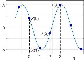
Figure 1: Consecutive periodically-spaced x(n) samples
of a real-valued sinusoidal sequence.

OK, let's consider three time-domain frequency estimation algorithms that estimate sinusoidal signal frequency based on the x(n) samples in Figure 1.

Real 3-Sample Frequency Estimation

DSP guru Clay Turner provides a method for estimating a real-valued sinusoid's frequency based on three time domain samples [1]. Turner's Real 3-Sample algorithm is:

   Real 3-Sample:   $f = \frac{f_s}{2\pi} cos^{-1}(\frac{x(0)+x(2)}{2x(1)}) \tag{1}$

After experimenting with Eq. (1) I learned it can give correct results assuming the 3-Sample x(n) input sequence satisfies the following restrictions:

* x(n) samples are real-valued and noise free,
* Nyquist sampling criterion is satisfied,
* Peak amplitude of x(n) is constant,
* DC component of x(n) is zero,
* Sample x(1) is not equal to zero.

Real 4-Sample Frequency Estimation

Turner also provides a method for estimating a real-valued sinusoid's frequency based on four time domain samples [2]. Turner's Real 4-Sample algorithm is:

Real 4-Sample: $f = \frac{f_s}{2\pi} \cdot cos^{-1}[\frac{1}{2}(\frac{x(3)-x(0)}{x(2)-x(1)}-1)] \tag{2}$

Equation (2) can provide correct results assuming the 4-Sample x(n) input sequence satisfies the following restrictions:

* x(n) samples are real-valued and noise free,
* Nyquist sampling criterion is satisfied,
* Peak amplitude of x(n) is constant,
* x(1) ≠ x(2).

Unlike Eq. (1), the Eq. (2) method can be applied when the x(n) sequence rides on a DC bias.

Complex 2-Sample Frequency Estimation

DSP wizard Dirk Bell recently showed me his two-sample method for estimating the frequency of a complex-valued noise-free sinusoid (reminiscent of complex-valued FM demodulation methods). Bell's algorithm to compute frequency f is:

$$ f = (\frac{f_s}{2\pi}) \cdot tan^{-1}[imag(x(n) \cdot x(n-1)^*)/real(x(n) \cdot x(n-1)^*)] \tag{3}$$

where the '*' symbol means conjugate. The derivation of Eq. (3) is given in Appendix A. Equation (3) can provide correct results assuming the complex $x(n)$ input sequence satisfies the following restrictions:

* $x(n) = Me^{j2\pi nf/f_s}$ and noise free,
* Nyquist sampling criterion is satisfied.

An Important Note

Notice that the mathematical derivations of our three algorithms could be called "exact." And by exact I mean no mathematical approximations, such as $ sin(x) = x $ for small $ x $, were used in their derivations. 

Algorithm Performance

The three time-domain frequency estimation algorithms work well when the input sinusoid is noise free. However, sadly, the Real 3-Sample and Real 4-Sample algorithms do not work well at all if the real-valued input sinusoid is contaminated with noise. (Clay Turner never claimed otherwise.) Figure 2 shows the performance of our three algorithms, for 500 individual frequency estimations, when the 700 Hz input sinusoids have a relatively high signal to noise ratio (SNR) of 60 dB.

My "noise" is standard garden variety, wideband, Gaussian-distributed, zero-mean, random noise samples. (The noise sequences used for the real and imaginary parts of the Complex 2-Sample algorithm input signal are independent of each other.) And my definition of input signal SNR is the traditional: $ SNR = 10log_{10}(signal variance/noise variance)$.

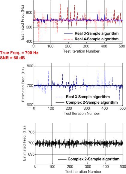
Figure 2: Algorithms' frequency estimation performances when the
input sinusoid's frequency is 700 Hz (fs = 8000 Hz)
with an SNR of 60 dB.

Look carefully at the vertical axes' values when comparing the Figure 2 frequency estimation results. In Figure 2 we see the Real 3-Sample and Real 4-Sample algorithms are very poor at frequency estimation when the input sinusoid is contaminated with noise. (The above Figure 2 performance measurements were made with both 16-bit and floating-point numbers. Those two number formats had essentially the same poor performance.)

Figure 2 also shows us the Complex 2-Sample algorithm produces moderately accurate results when the input sinusoid's SNR is 60 dB. Appendix B presents the three algorithms' performances when the input sinusoid's SNR is less than 60 dB.

Software Modeling

If you decide to model the performance of the above Eq. (1) and Eq. (2) algorithms with noise-contaminated real sinusoids, be aware that those methods can produce invalid complex-valued frequency estimates that should be ignored. That happens when the arguments of the $cos^{-1}()$ functions are, due to noisy $ x(n) $ samples, greater than unity. You'll often see this situation when the input sinusoids are low-SNR or low-frequency (relative to the Fs sample rate).

Conclusions

I've presented three sinusoidal frequency estimation algorithms, Eqs. (1), (2), and (3), that use time-domain samples as opposed to FFT frequency-domain samples. Those algorithms only provide correct frequency estimation results for ideal noise-free input sinusoids. As such, those algorithms are mostly of academic interest only. (No one claimed those algorithms were of significant practical value.) My thoughts on the problems encountered when using the three algorithms in practical DSP applications are given in Appendix C.

One point I want to make here is this: Although the Real 3-Sample and Real 4-Sample frequency estimation algorithms are mathematically exact, their performance is very poor in the presence of noise. Thus it is risky to assume that mathematically exact DSP algorithms will always be useful in real-world practical signal processing applications .

April 30, 2017 Update: I've continued to learn more about the above Eq. (3). As it turns out, that algorithm is described in the literature of "frequency estimation" and it goes by the name of the "Lank-Reed-Pollon algorithm." In my initial software modeling of Eq. (3) it appeared to me that it provided an unbiased estimate of the frequency of a complex-valued sinusoid. After more thorough modeling I've learned that Eq. (3) is indeed a biased estimator when the input complex-valued sinusoid has a low SNR and is either low in frequency (near zero Hz) or high in frequency (near Fs/2 Hz). This is important because it means that averaging multiple frequency estimation values does not necessarily improve our final frequency estimate's accuracy

Acknowledgment

I thank Dirk Bell for his very useful suggestions regarding the first draft of this blog. I also thank Cedron Dawg for correcting a notational error in the original version of Appendix A.

References

[1] Clay Turner, http://www.claysturner.com/dsp/3pointfrequency.pdf
[2] Clay Turner, http://www.claysturner.com/dsp/4pointfrequency.pdf

Appendix A: Derivation of Eq. (3)

Dirk Bell's derivation of his Eq. (3) expression proceeds as follows: Assume the complex-valued sinusoid of frequency $ f $ is described by:

We can, where the '*' symbol means conjugation, write:

The radian angle of product P is:

$$ arg(P) = 2\pi f/f_s $$ $$ = tan^{-1}[imag(x(n) \cdot x(n-1)^*)/real(x(n) \cdot x(n-1)^*)].$$

Arbitrarily assuming index $ n = 1 $, our desired expression for $ f $ is:

$$ f = (\frac{f_s}{2\pi}) \cdot tan^{-1}[imag(P)/real(P)] $$ $$ = (\frac{f_s}{2\pi}) \cdot tan^{-1}[imag(x(n) \cdot x(n-1)^*)/real(x(n) \cdot x(n-1)^*)].$$

Appendix B: Algorithms' Performances With Low SNR Input Signals

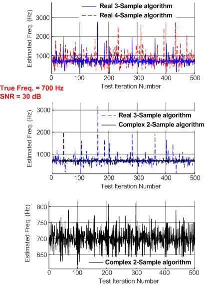
Figure B-1: Algorithms' frequency estimation performances when the
input sinusoid's frequency is 700 Hz (fs = 8000 Hz)
with a signal SNR of 30 dB.

Figure B-2 shows the performance of the Real 3-Sample and Complex 2-Sample algorithms, for 500 individual frequency estimations, when the 700 Hz input sinusoids have an SNR of 10 dB. (For reference, the top panel of Figure B-2 shows the difference between a noise-free 700 Hz sinusoid and an SNR = 10 dB sinusoid.) In this scenario the two algorithms have terribly poor performance.

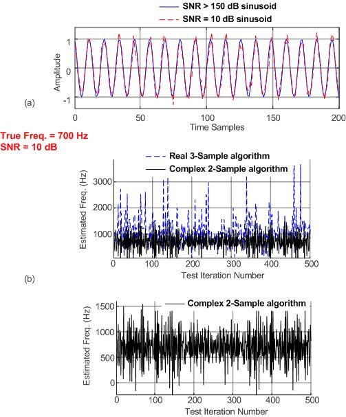
Figure B-2: Algorithm performance: (a) comparison of a noise-free
and a noisy input sinusoid; (b) algorithms' frequency
estimation performances when the input sinusoid's
frequency is 700 Hz (fs = 8000 Hz) with a signal SNR of 10 dB.

Appendix C: Practical Problems of the Three Frequency Estimation Algorithms

According to my software modeling, in the presence of noise the Real 3-Sample and Real 4-Sample algorithms typically produce biased results (i.e., the mean of multiple frequency estimations is usually greater then the true input signal's frequency). Thus averaging the results of multiple frequency estimations is not guaranteed to improve their performances. An input signal SNR of roughly 40 dB combined with multiple results averaging is necessary for those algorithms to be just marginally useful. There's more bad news. When the input signal's frequency is less than fs/20 Hz the Real 3-Sample and Real 4-Sample algorithms provide wildly incorrect results.

Unlike the Real 3-Sample algorithm, the Real 4-Sample's performance is not degraded by a DC bias on the input sinusoid but it requires a much higher input signal SNR to achieve comparable performance with the Real 3-Sample algorithm.

The Complex 2-Sample algorithm provides unbiased frequency estimation results, even at low input signal frequencies. So averaging multiple Complex 2-Sample output samples will improve this algorithm's performance. While its performance is superior to the Real 3-Sample and Real 4-Sample algorithms, the disadvantage of the Complex 2-Sample algorithm is that it requires a complex-valued input. So real-valued input sequences must be converted to an analytic complex-valued sequence before the frequency estimation process can begin.

To be truly useful when their input sinusoids are contaminated by noise and narrowband interfering spectral components, our three frequency estimation methods need to be preceded by some sort of SNR-enhancing narrow bandpass filtering.

Sign in