Wave Equation in Higher Dimensions

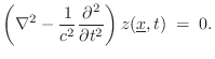
Free Books Physical Audio Signal Processing

The wave equation in 1D, 2D, or 3D may be written as

$\displaystyle \left(\nabla ^2 - \frac{1}{c^2}\frac{\partial^2}{\partial t^2} \right) z(\underline{x},t) \eqsp 0, \protect$

(B.47)

where, in 3D, $z(\underline{x},t)$ denotes the amplitude of the wave at time

and position $\underline{x}\in{\bf R}^3$ , and

$\displaystyle \nabla ^2 \isdefs \nabla \cdot \nabla \isdefs \nabla ^T\nabla \eq... ...tial x^2} + \frac{\partial^2}{\partial y^2} + \frac{\partial^2}{\partial z^2}$

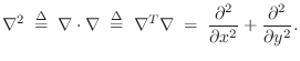
denotes the Laplacian operator in Euclidean coordinates. (In general coordinates, it is often denoted by $\Delta$ .) To investigate solutions of the wave equation, as pursued in §B.8.3 below, it is useful to first develop some simple expressions and notations for elementary waves in 2D and 3D.

Plane Waves in Air

Figure B.9 shows a 2D cross-section of a snapshot (in time) of the sinusoidal plane wave

$\displaystyle p(x,y,z) = p_0 + \cos(k_x x + k_y y)$

for $k_x = 2\pi 5$ and $k_y=2\pi 5/2$ , with

and

in the range

**Figure:** Gray-scale density plot of the cross-section of a sinusoidal plane wave $p(t,\underline{x}) = \cos\left(\omega t - \underline{k}^T\underline{x}\right)$ , at with vector wavenumber $\underline{k}^T=[10\pi, 5\pi, 0]$ .
$\includegraphics[width=\twidth]{eps/planewave}$

Figure B.10 depicts a more mathematical schematic of a sinusoidal plane wave traveling toward the upper-right of the figure. The dotted lines indicate the crests (peak amplitude location) along the wave.

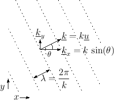
**Figure:** Wave crests of the sinusoidal traveling plane wave $p(t,\underline{x}) = \cos\left(\omega t - \underline{k}^T\underline{x}\right)$ , for some fixed time and $\underline{x}$ in the plane.
$\includegraphics{eps/planewaveangle}$

The direction of travel and spatial frequency are indicated by the vector wavenumber $\underline{k}$ , as discussed in in the following section.

Vector Wavenumber

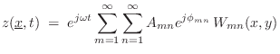
Mathematically, a sinusoidal plane wave, as in Fig.B.9 or Fig.B.10, can be written as

$\displaystyle p(t,\underline{x}) \eqsp p_0 + A\cos\left(\omega t - \underline{k}^T\underline{x}+ \phi\right), \quad \underline{x}\in{\bf R}^3 \protect$

(B.48)

where p(t,x) is the pressure at time

(seconds) and position $\underline{x}\in{\bf R}^3$ (3D Euclidean space). The amplitude

, phase $\phi$ , and radian frequency $\omega$ are ordinary sinusoid parameters [451], and $\underline{k}$ is the vector wavenumber:

$\displaystyle \underline{k}\eqsp \left[\begin{array}{c} k_x \\ [2pt] k_y \\ [2p... ... \cos{\beta} \\ [2pt] \cos{\gamma}\end{array}\right] \isdefs k\,\underline{u},$

where

$\underline{u}=$ (unit) vector of direction cosines
$k = 2\pi/\lambda =$ (scalar) wavenumber along travel direction

Thus, the vector wavenumber $\underline{k}= k\,\underline{u}$ contains

wavenumber along the travel direction in its magnitude $k=\left\Vert\,\underline{k}\,\right\Vert$
travel direction in its orientation $\underline{u}= \underline{k}/k$

Note that wavenumber units are radians per meter (spatial radian frequency).

To see that the vector wavenumber $\underline{k}= k\,\underline{u}$ has the claimed properties, consider that the orthogonal projection of any vector $\underline{x}$ onto a vector collinear with $\underline{u}$ is given by $(\underline{u}^T\underline{x})\underline{u}$ [451].^B.35Thus, $(\underline{u}^T\underline{x})\underline{u}$ is the component of $\underline{x}$ lying along the direction of wave propagation indicated by $\underline{u}$ . The norm of this component is $\vert\vert\,(\underline{u}^T\underline{x})\underline{u}\,\vert\vert =\vert\underline{u}^T\underline{x}\vert$ , since $\underline{u}$ is unit-norm by construction. More generally, $\underline{u}^T\underline{x}$ is the signed length (in meters) of the component of $\underline{x}$ along $\underline{u}$ . This length times wavenumber gives the spatial phase advance along the wave, or, $\theta(\underline{x})=k\cdot(\underline{u}^T\underline{x}) \isdeftext \underline{k}^T\underline{x}$ .

For another point of view, consider the plane wave $\cos(\underline{k}^T\underline{x})$ , which is the varying portion of the general plane-wave of Eq. $\,$ (B.48) at time , with unit amplitude and zero phase $\phi=0$ . The spatial phase of this plane wave is given by

$\displaystyle \theta(\underline{x}) \isdefs \underline{k}^T\underline{x}\eqsp k_x x + k_y y + k_z z.$

Recall that the general equation for a plane in 3D space is

$\displaystyle \alpha x + \beta y + \gamma z =$ constant

where $\alpha$ , $\beta$ , and $\gamma$ are real constants, and

, and

are 3D spatial coordinates. Thus, the set of all points $\underline{x}^T=(x,y,z)$ yielding the same value $\theta(\underline{x})=\theta_0$ define a plane of constant phase $\theta_0$ in ${\bf R}^3$ .

As we know from elementary vector calculus, the direction of maximum phase advance is given by the gradient of the phase $\theta(\underline{x})$ :

$\displaystyle \underline{\nabla }\theta(\underline{x}) \isdefs \left[\begin{ar... ...rray}{c} k_x \\ [2pt] k_y \\ [2pt] k_z\end{array}\right] \isdefs \underline{k}$

This shows that the vector wavenumber $\underline{k}$ is equal to the gradient of the phase $\theta(\underline{x})$ , so that $\underline{k}$ points in the direction of maximum spatial-phase advance.

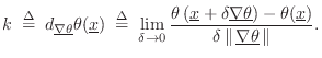
Since the wavenumber is the spatial frequency (in radians per meter) along the direction of travel, we should be able to compute it as the directional derivative of $\theta(\underline{x})$ along $\underline{k}$ , i.e.,

$\displaystyle k \isdefs d_{\underline{\nabla \theta}}\theta(\underline{x}) \isd... ...ta(\underline{x})}{\delta \left\Vert\,\underline{\nabla \theta}\,\right\Vert}.$

An explicit calculation yields

$\displaystyle k \eqsp \left\Vert\,\underline{\nabla \theta}\,\right\Vert \eqsp \sqrt{k_x^2+k_y^2+k_z^2} \isdefs \left\Vert\,\underline{k}\,\right\Vert$

as needed.

Scattering of plane waves is discussed in §C.8.1.

Solving the 2D Wave Equation

Since solving the wave equation in 2D has all the essential features of the 3D case, we will look at the 2D case in this section.

Specializing Eq. $\,$ (B.47) to 2D, the 2D wave equation may be written as

$\displaystyle \left(\nabla ^2 - \frac{1}{c^2}\frac{\partial^2}{\partial t^2} \right) z(\underline{x},t) \eqsp 0.$

where

$\displaystyle \nabla ^2 \isdefs \nabla \cdot \nabla \isdefs \nabla ^T\nabla \eqsp \frac{\partial^2}{\partial x^2} + \frac{\partial^2}{\partial y^2}.$

The 2D wave equation is obeyed by traveling sinusoidal plane waves having any amplitude , radian frequency $\omega$ , phase $\phi$ , and direction $\underline{u}$ :

$\displaystyle z(\underline{x},t) = A\,e^{j\phi}\,e^{j(\omega t - \underline{k}^T\underline{x})}$

where $\underline{k}=k\underline{u}$ denotes the vector-wavenumber, $k=\omega/c$ denotes the wavenumber (spatial radian frequency) of the wave along its direction of travel, and $\underline{u}$ is a unit vector of direction cosines. This is the analytic-signal form of a sinusoidal traveling plane wave, and we may define the real (physical) signal as the real part of the analytic signal, as usual [451]. We see that the only constraint imposed by the wave equation on this general traveling-wave is the so-called dispersion relation:

$\displaystyle k\eqsp \vert\underline{k}\vert\eqsp \frac{\omega}{c}$

In particular, the wave can travel in any direction, with any amplitude, frequency, and phase. The only constraint is that its spatial frequency

is tied to its temporal frequency $\omega$ by the dispersion relation.^B.36

The sum of two such waves traveling in opposite directions with the same amplitude and frequency produces a standing wave. For example, if the waves are traveling parallel to the axis, we have

$\displaystyle z(\underline{x},t) \eqsp A\,e^{j\phi}\,e^{j\omega t - kx} + A\,e^{j\phi}\,e^{j\omega t + kx} \eqsp 2A\,e^{j(\omega t + \phi)}\,\cos(kx) \protect$

(B.49)

which is a standing wave along

2D Boundary Conditions

We often wish to find solutions of the 2D wave equation that obey certain known boundary conditions. An example is transverse waves on an ideal elastic membrane, rigidly clamped on its boundary to form a rectangle with dimensions $X\times Y$ meters.

Similar to the derivation of Eq. $\,$ (B.49), we can subtract the second sinusoidal traveling wave from the first to yield

$\displaystyle z(\underline{x},t) \eqsp A\,e^{j\phi}\,e^{j\omega t - kx} - A\,e^{j\phi}\,e^{j\omega t + kx} \eqsp 2A\,e^{j(\omega t + \phi+\pi/2)}\,\sin(kx)$

which satisfies the zero-displacement boundary condition along the

axis. If we restrict the wavenumber

to the set $m\pi/X$ , where

is any positive integer, then we also satisfy the boundary condition along the line parallel to the

axis at

. Similar standing waves along

will satisfy both boundary conditions along

and

Note that we can also use products of horizontal and vertical standing waves

$\displaystyle z(\underline{x},t) \eqsp A\,e^{j\omega t + \phi}\,\sin(kx)\sin(ky)$

because, when taking the partial derivative with respect to

, the term $\sin(ky)$ is simply part of the constant coefficient, and vice versa.

To build solutions to the wave equation that obey all of the boundary conditions, we can form linear combinations of the above standing-wave products having zero displacement (``nodes'') along all four boundary lines:

$\displaystyle z(\underline{x},t) \eqsp e^{j\omega t} \sum_{m=1}^{\infty}\sum_{n=1}^{\infty} A_{mn}e^{j\phi_{mn}}\,W_{mn}(x,y) \protect$

(B.50)

where

$\displaystyle W_{mn}(x,y) \isdefs \sin\left(m\frac{\pi}{X}x\right)\sin\left(n\frac{\pi}{Y}y\right).$

By construction, all linear combinations of the form Eq. $\,$ (B.50) are solutions of the wave equation that satisfy the zero boundary conditions along the rectangle

. Since sinusoids at different frequencies are orthogonal, the solution building-blocks $W_{mn}(x,y)$ are orthogonal under the inner product

$\displaystyle \left<f,g\right> \isdefs \int_0^X\int_0^Y f(x,y)\overline{g}(x,y)\,dx\,dy.$

It remains to be shown that the set of functions $W_{mn}(x,y)$ is complete, that is, that they form a basis for the set of all solutions to the wave equation satisfying the boundary conditions. Given that, we can solve the problem of arbitrary initial conditions. That is, given any initial

over the membrane (subject to the boundary conditions, of course), we can find the amplitude of each excited mode by simple projection:

$\displaystyle Z_{mn} \isdef \frac{\left<z,W\right>}{\left<W,W\right>}$

Showing completeness of the basis $W_{mn}(x,y)$ in the desired solution space is a special case (zero boundary conditions) of the problem of showing that the 2D Fourier series expansion is complete in the space of all continuous rectangular surfaces.

The Wikipedia page (as of 1/31/10) on the Helmholtz equation provides a nice ``entry point'' on the above topics and further information.

3D Sound

The mathematics of 3D sound is quite elementary, as we will see below. The hard part of the theory of practical systems typically lies in the mathematical approximation to the ideal case. Examples include Ambisonics [158] and wave field synthesis [49].

Consider a point source at position $\underline{x}_s\in{\bf R}^3$ . Then the acoustic complex amplitude at position $\underline{x}_l\in{\bf R}^3$ is given by

$\displaystyle p(\underline{x}_l;\underline{x}_s) = p_1(\underline{x}_s) \frac{e... ...derline{x}_l-\underline{x}_s\vert}}{\vert\underline{x}_l-\underline{x}_s\vert}$

where $p_1(\underline{x}_s)$ denotes the complex amplitude one meter from the point source in any direction, and $k=2\pi/\lambda$ denotes the wavenumber (spatial radian frequency). Distributed acoustic sources are handled as a superposition of point sources, so the point source is a completely general building block for all types of sources in linear acoustics.

The fundamental approximation problem in 3D sound is to approximate the complex acoustic field at one or more listening points using a finite set of loudspeakers, which are often modeled as a point source for each speaker.

Next Section:
The Ideal Vibrating String
Previous Section:
Properties of Gases