Solving the 2D Wave Equation
Since solving the wave equation in 2D has all the essential features of the 3D case, we will look at the 2D case in this section.
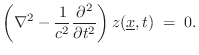
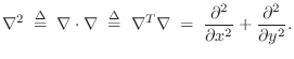
Specializing Eq.![]() (B.47) to 2D, the 2D wave equation may
be written as
(B.47) to 2D, the 2D wave equation may
be written as
The 2D wave equation is obeyed by traveling sinusoidal plane
waves having any amplitude ![]() , radian frequency
, radian frequency ![]() , phase
, phase
![]() , and direction
, and direction
![]() :
:
The sum of two such waves traveling in opposite directions with the
same amplitude and frequency produces a standing wave. For example,
if the waves are traveling parallel to the ![]() axis, we have
axis, we have
which is a standing wave along
Next Section:
2D Boundary Conditions
Previous Section:
Vector Wavenumber