Filtering Noise: The Basics (Part 1)

• Basics
• Python
• Probability

Introduction

Finding signals in the presence of noise is one of the fundamental quests of the discipline of signal processing. Noise is inherently random by nature, so a probability oriented approach is needed to develop a mathematical framework for filtering (i.e. removing/suppressing) noise. This framework or discipline, formally referred to as stochastic signal processing, is often taught in graduate level engineering programs and is covered from different perspectives in excellent texts such as [1][2] and numerous online courses (check out some of this free course material). In this introductory level blog post, I would like to derive some of the basic results in this vast field from first principles and in the process help the reader develop an intuitive understanding of the underlying concepts. In the interest of readability, I have split the material over multiple posts. Here is part 1.

Let us consider a discrete-time noise process. This can be thought of as a sequence ${w[n]}$, where $n$ is the sample or time index. Each element or sample in this sequence is a random value following a certain probability distribution. A commonly encountered scenario is one where $w[n]$ follows a Gaussian or normal distribution with zero mean and variance $\sigma^2$, denoted $\mathcal{N}(0, \sigma^2)$. This is a pretty good model for additive sensor noise in a measurement system or electronic circuit noise in a digital communication system, for example. Let us assume that each $w[n]$ follows the same distribution, i.e. for the Gaussian noise case, the variance $\sigma^2$ is independent of $n$ (this is called a stationary process, in case you want to read up more). In such a model, the noise samples are said to be independent and identically distributed, or i.i.d. for short. Such a noise process is also referred to as white noise, because when viewed in frequency domain, it is comprised of equal contributions from all frequencies (an analogy to white light, which is a made of all colors combined together in equal proportion).

Intuitively, when dealing with signals corrupted by the additive noise process (i.e. observed signal = true signal + noise) of the type described above, "averaging" seems like a pretty good strategy for reducing the contribution of the noise. The basic idea is that averaging a bunch of random noise samples which statistically have a mean of zero should result in something close to "zero". Of course, the result of averaging is highly unlikely to be precisely zero, but will tend to zero as more and more samples are averaged (for a precise definition of "tend to", check out the well known Law of Large Numbers). In signal processing terminology, this averaging operation is referred to as low-pass filtering or smoothing. This can be accomplished using linear filters (our focus here) or a host of non-linear techniques. In fact, the simplest manifestation of averaging you can imagine, i.e. taking an equally weighted average of $K$ noise samples, is a special case of a finite impulse response (FIR) filter, which we will discuss next.

FIR filters

An FIR filter is a basic structural element in DSP. Given an input signal $w[n]$ and a set of $K$  FIR filter coefficients ${h[k], \; k=0, \ldots, K-1}$, the output of the filter $y[n]$ when it acts on the input signal is given by:

$y[n] = \sum_{k=0}^{K-1} h[k] w[n-k]$, denoted $y = h \star x$ (convolution)

Statistical properties of the filter output

Since the input to the filter is a random process, the output can also be viewed as a random process. Let us calculate the mean and variance of the output signal when the input $w[n]$ is an i.i.d. sequence, with each sample distributed as $\mathcal{N} (0, \sigma^2)$ (white Gaussian noise, as discussed above). Since expectation (denoted $\mathbb{E}(\cdot)$) is a linear operation ($\mathbb{E}(ax+by) = a\mathbb{E}(x) + b\mathbb{E}(y)$), the mean or expected value of $y[n]$ is 0.

$\mathbb{E}(y[n]) = \mathbb{E} \left(  \sum_{k=0}^{K-1} h[k] w[n-k] \right) =  \sum_{k=0}^{K-1} h[k] \underbrace{\mathbb{E}(w[n-k])}_{=0} =   0$

The variance, by definition, is given by $\sigma_Y^2 = \mathbb{E}(y[n]^2) - \left( \mathbb{E} (y[n]) \right)^2 =  \mathbb{E} (y[n]^2)$, since we have already established that $\mathbb{E} (y[n]) = 0$. Let us simplify this expression:

$\sigma_Y^2 = \mathbb{E} \left( \sum_{k=0}^{K-1} h[k]w[n-k] \right)^2$

$\;\;\;\; = \mathbb{E} \left( \sum_{k=0}^{K-1} \sum_{k'=0}^{K-1} h[k] h[k'] w[n-k] w[n-k'] \right)$

$\;\;\;\; = \sum_{k=0}^{K-1} \sum_{k'=0}^{K-1} h[k] h[k'] \mathbb{E} (w[n-k] w[n-k']) $

At this point we need a new concept. We previously defined the statistics of each sample $w[n]$, but did not say anything explicit about the joint statistics of $w[n]$ and $w[m]$ for $n \neq m$. However, we did assume that the noise samples were independent of each other. This effectively translates to the following property: 

$\mathbb{E} (w[n]w[m]) = \mathbb{E} (w[n]) \mathbb{E} (w[m]) = 0$ if $n \neq m$. However, when $m=n$, $\mathbb{E} (w[n]w[m]) = \mathbb{E}(w[n]^2) = \sigma^2$, by definition. The quantity we just computed, viz. $\mathbb{E} (w[n]w[m])$ is known as the auto-correlation. 

Using these properties of the auto-correlation, we can simplify:

$\sigma_Y^2 =    \underbrace{ \sum_{k=0}^{K-1} \sum_{k'=0}^{K-1} }_{k=k'} h[k] h[k'] \mathbb{E}(w[n-k] w[n-k'] )$

$ \;\;\;\;+  \underbrace{\sum_{k=0}^{K-1} \sum_{k'=0}^{K-1} }_{k \neq k'} h[k] h[k'] \mathbb{E} (w[n-k] w[n-k'])$

$ \;\;\;\; = \mathbb{E} \sum_{k=0}^{K-1} h[k]^2 \sigma^2 + \sum_{k=0}^{K-1} \sum_{k'=0}^{K-1} h[k] h[k'] \cdot 0$

$ \;\;\;\; = \sigma^2 \sum_{k=0}^{K-1} h[k]^2$

This is a nice, clean result. In plain English, the variance of the output signal is the variance of the input signal multiplied by the sum of the energy in all the filter taps. As an aside, using Parseval's theorem, one can relate this expression to the energy of the filter in frequency domain. 

So is computing mean and variance of the output adequate? In this case, since the input $w$ is normally distributed, and all we did was apply a linear filter to it, the output is normally distributed as well (a linear combination of Gaussian random variables is also Gaussian, as shown in the Appendix for a special case), which means that each individual output sample is fully characterized by it's mean and variance.

What about the relation between different samples of the output, $y[n]$ and $y[m]$, as captured by the auto-correlation $R_{YY}(n,m) = \mathbb{E} (y[n]y[m])$? Recall that we had stated earlier (albeit without proof) that the auto-correlation of the input is 0 when $n \neq m$. This will not be the case at the output of the filter. Since each output is computed as a linear combination of $K$ inputs, you can expect the output samples to have some correlation with each other. Let us now compute a mathematical expression for that. 

$\mathbb{E} (y[n]y[m]) = \sum_{k=0}^{K-1} \sum_{k'=0}^{K-1} h[k] h[k'] \mathbb{E} (w[n-k] w[m-k'])$

$ \;\;\;\; = \sigma^2 \sum_{k=0}^{K-1} h[k] h[m-n+k]$

The last step follows because $\mathbb{E} (w[n-k] w[m-k'])$ is non-zero (and equal to $\sigma^2$) only when $n-k=m-k'$. 

Let us look at a couple of interesting properties of $R_{YY}$ here, though this material deserves a more elaborate discussion:

- The auto-correlation $R_{YY}(n,m)$ is a function of $(n-m)$ and does not depend on the individual values of $n$ and $m$. Such a process is said to be wide-sense stationary (a special case of the aforementioned stationary process).

- $R_{YY}(n,m) \equiv R_{YY}(n-m)$ can be massaged and expressed as $h[k] \star h[-k]$, i.e. the convolution of the filter taps with their time-reversed or flipped version. As a result, in frequency domain, the Fourier transform of the auto-correlation (known as power spectral density) becomes a product of the Fourier transform of the filter taps with it's conjugate.

Noise suppression with FIR filters

Let us now focus on the noise suppression properties of FIR filters. We know that the output variance is $\sigma^2 \sum_{k=0}^{K-1} h(k)^2$, which is less than the input variance $\sigma^2$ if $\sum_{k=0}^{K-1} h(k)^2 < 1$. But how well can we do? If we impose the constraint $\sum_{k=0}^{K-1} h(k) = 1$, i.e. the DC level of the output is same as the input (this is a reasonable constraint to impose on the signal of interest, which allows us to compare the noise variance before/after filtering without worrying about scaling factors), the choice of filter coefficients that minimize the output noise variance can be stated as this optimization problem:

Find $h[k], \; k=0,\ldots,K-1$ which minimize $\sigma^2 \sum_{k=0}^{K-1} h(k)^2$, subject to $\sum_{k=0}^{K-1} h(k) = 1$. 

The problem can be formally solved using the technique of Lagrange multipliers (see Appendix), but it is clear by inspection that $h[k] = 1/K \; \forall \; k$ is the optimal solution. This is the commonly known moving average or boxcar (thanks to its shape) filter. Intuitively, it makes sense that if all the noise samples are statistically the same, each one of them should be given an equal weight in an averaging based noise reduction scheme.

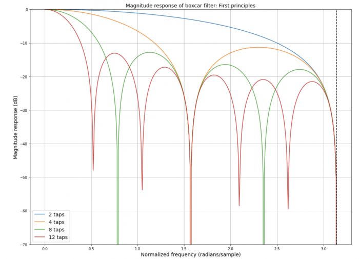
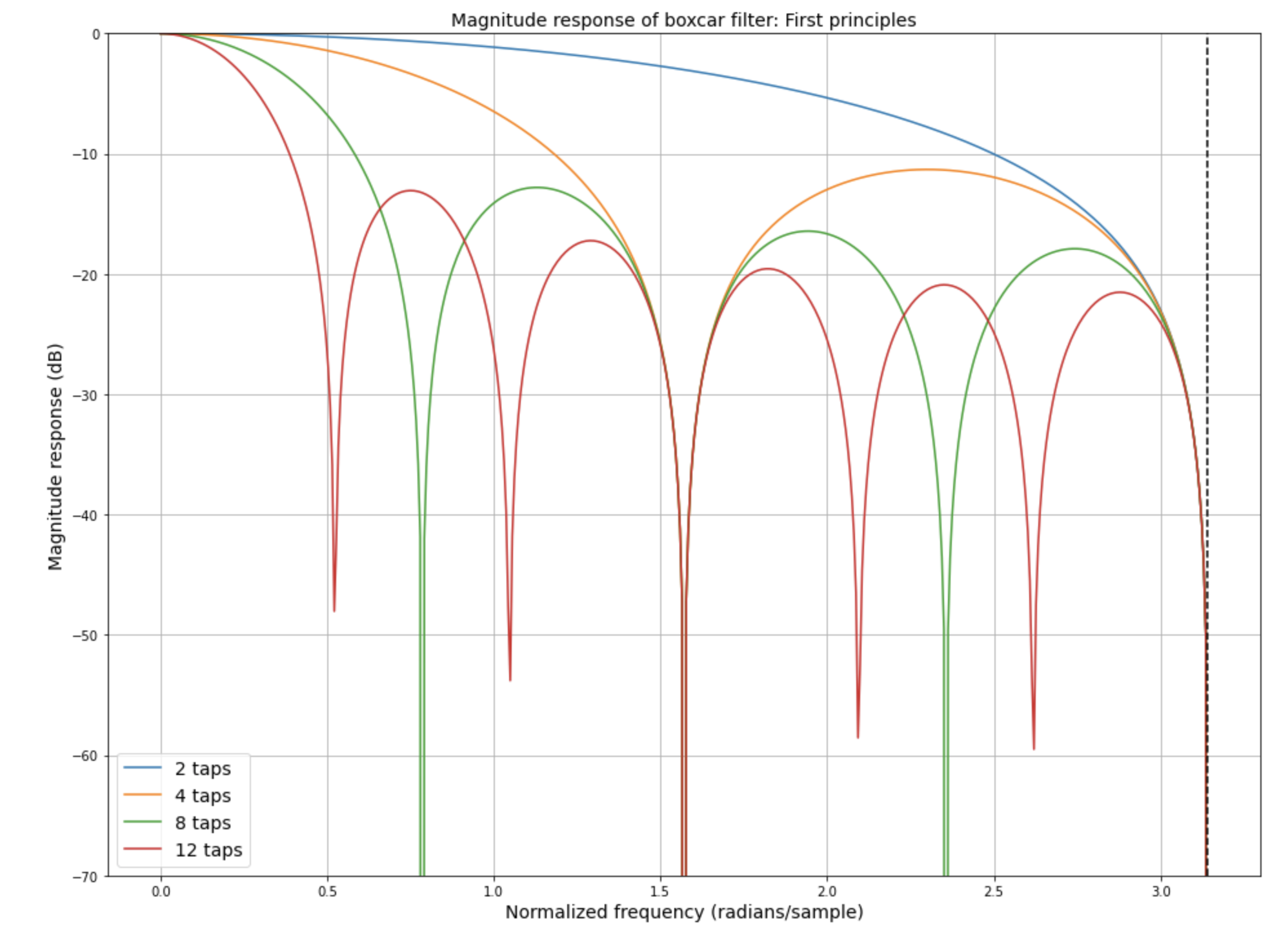
Why is it that signal processing practitioners are often reluctant to deploy the boxcar filter, given that it is the optimal filter for suppressing additive white noise (for a fixed number of filter taps)? To answer that, it is best to look at this filter in frequency domain. The frequency response of the filter (the sinc function) has large side lobes. This means that higher frequency components of the signal are poorly suppressed and would in fact fold back into the spectrum of interest if the filtered signal were to be downsampled. Also, the shape of the filter in the passband (roughly speaking, the low frequency region of interest) is rather sharp, which means that different frequencies in the signal will be attenuated differently (this could be a deal breaker, depending on the application at hand).

Better filters can certainly be designed, which come close to the boxcar in terms of noise suppression, while achieving much more attractive properties in frequency domain. One such design approach is the windowed method. You can explore the concepts further here and here. I will add a numerical example in a later post. In the meantime, take a look at this simple Jupyter notebook to explore the frequency domain behavior of boxcar filters from first principles and also based on the scipy package in Python. 

Shown below is a sample output of the notebook. What do you notice about the location of the first null and the number of side lobes as a function of the number of taps in the boxcar filter?

In the next post, I will explore the noise suppression properties of a simple infinite impulse response filter.

Appendix

Sum of two independent Gaussian random variables

Let us show that the sum of two independent random variables with Gaussian distribution (zero mean, unit variance) is also Gaussian. The proof can be easily extended to cover weighted sums of more than two independent Gaussian random variables (possibly with unequal means and variances).

We will rely on the fact that the probability density of the sum of two independent random variables can be written as the convolution of their individual probability density functions. In our special case, 

$Z = X+Y$,

where $X$ and $Y$ are both $\mathcal{N}(0, 1)$. The probability density function of $X$ and $Y$ is (by definition) specified as

$f(x) = \frac{1}{\sqrt{2 \pi}} e^{- \frac{x^2}{2} }$

The probability density function of $Z$ is given by $f_Z = f \star f$, i.e.

$f_Z(z) = \int_{-\infty}^{\infty} f(x) f(z-x) dx$

$\;\;\;\; =  \frac{1}{2 \pi} \int_{-\infty}^{\infty} e^{- \frac{x^2}{2} } e^{- \frac{(z-x)^2}{2} } $

Lagrange multiplier formulation for finding ideal FIR filter taps

Recall the optimization problem: Find $h[k], \; k=0,\ldots,K-1$ which minimize $\sigma^2 \sum_{k=0}^{K-1} h[k]^2$, subject to $\sum_{k=0}^{K-1} h(k) = 1$. 

The technique of Lagrange multipliers is often used to solve this type of constrained optimization problem. Let us introduce a Lagrange multiplier $\lambda$ and write our objective function as

$\Phi(h, \lambda) = \sigma^2 \sum_{k=0}^{K-1} h[k]^2 + \lambda \left( \sum_{k=0}^{K-1} h[k] -1 \right)$

Now we have an unconstrained optimization problem, which is to find $\{h[k]\}$ and $\lambda$ that minimize $\Phi(h, \lambda)$. Let us compute the partial derivatives of $\Phi$ with respect to $h[k]$ and $\lambda$ and set them to 0.

$\frac{\partial \Phi}{\partial h[k]} = 2 \sigma^2 h[k] + \lambda = 0$

$\frac{\partial \Phi}{\partial \lambda} = \sum_{k=0}^{K-1} h[k] - 1 = 0$

The above equations imply $h[k] = -\frac{\lambda}{2 \sigma^2} \; \forall \; k$ and $-K \frac{\lambda}{2 \sigma^2} = 1$. Putting them together we get $h[k] = 1/K \; \forall \; k$.

References

[1] S. Karlin and H. Taylor, "A First Course in Stochastic Processes", Academic Press, 1975

[2] A.Papoulis, "Probability, Random Variables, and Stochastic Processes", McGraw Hill, 2002

Sign in