Two Coupled Strings
Two Ideal Strings Coupled at an Impedance
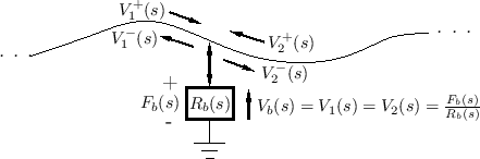
A diagram for the two-string case is shown in
Fig. C.30. This situation is a special case of the
loaded waveguide junction, Eq.![]() (C.98), with the
number of waveguides being
(C.98), with the
number of waveguides being ![]() , and the junction load being the
transverse driving-point impedance
, and the junction load being the
transverse driving-point impedance ![]() where the string drives
the bridge. If the bridge is passive, then its impedance
where the string drives
the bridge. If the bridge is passive, then its impedance ![]() is
a positive real function (see §C.11.2). For a direct derivation,
we need only observe that (1) the string velocities of each string
endpoint must each be equal to the velocity of the bridge, or
is
a positive real function (see §C.11.2). For a direct derivation,
we need only observe that (1) the string velocities of each string
endpoint must each be equal to the velocity of the bridge, or
![]() , and (2) the sum of forces of both strings equals the force
applied to the bridge:
, and (2) the sum of forces of both strings equals the force
applied to the bridge:
![]() . The bridge impedance
relates the force and velocity of the bridge via
. The bridge impedance
relates the force and velocity of the bridge via
![]() . Expanding into traveling wave components in the Laplace
domain, we have
. Expanding into traveling wave components in the Laplace
domain, we have
| (C.108) | |||
| (C.109) | |||
| (C.110) | |||
| (C.111) |
or
Given the filter output ![]() , the outgoing traveling velocity waves are
given by
, the outgoing traveling velocity waves are
given by
| (C.112) | |||
| (C.113) |
Thus, the incoming waves are subtracted from the bridge velocity to get the outgoing waves.
Since
![]() when
when
![]() , and vice versa exchanging strings
, and vice versa exchanging strings ![]() and
and ![]() ,
, ![]() may be
interpreted as the transmission admittance filter associated with
the bridge coupling. It can also be interpreted as the bridge admittance
transfer function from every string, since its output is the bridge
velocity resulting from the sum of incident traveling force waves.
may be
interpreted as the transmission admittance filter associated with
the bridge coupling. It can also be interpreted as the bridge admittance
transfer function from every string, since its output is the bridge
velocity resulting from the sum of incident traveling force waves.
A general coupling matrix contains a filter transfer function in each
entry of the matrix. For ![]() strings, each conveying a single type of
wave (e.g., horizontally polarized), the general linear coupling
matrix would have
strings, each conveying a single type of
wave (e.g., horizontally polarized), the general linear coupling
matrix would have ![]() transfer-function entries. In the present
formulation, only one transmission filter is needed, and it is shared
by all the strings meeting at the bridge. It is easy to show that the
shared transmission filter for two coupled strings generalizes to
transfer-function entries. In the present
formulation, only one transmission filter is needed, and it is shared
by all the strings meeting at the bridge. It is easy to show that the
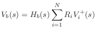
shared transmission filter for two coupled strings generalizes to ![]() strings coupled at a common bridge impedance: From
(C.98), we have
strings coupled at a common bridge impedance: From
(C.98), we have
The above sequence of operations is formally similar to the one multiply scattering junction frequently used in digital lattice filters [297]. In this context, it would be better termed the ``one-filter scattering termination.''
When the two strings are identical (as would be appropriate in a model for coupled piano strings), the computation of bridge velocity simplifies to
where

Note that a yielding bridge introduces losses into all attached
strings. Therefore, in a maximally simplified implementation, all
string loop filters (labeled
LPF![]() and
LPF
and
LPF![]() in
Fig.C.31) may be eliminated, resulting in only one
filter--the transmission filter--serving to provide all losses in a
coupled-string simulation. If that transmission filter has no
multiplies, then neither does the entire multi-string simulation.
in
Fig.C.31) may be eliminated, resulting in only one
filter--the transmission filter--serving to provide all losses in a
coupled-string simulation. If that transmission filter has no
multiplies, then neither does the entire multi-string simulation.
Coupled Strings Eigenanalysis
In §6.12.2, general coupling of horizontal and vertical planes of vibration in an ideal string was considered. This eigenanalysis will now be applied here to obtain formulas for the damping and mode tuning caused by the coupling of two identical strings at a bridge. This is the case that arises in pianos [543].
The general formula for linear, time-invariant coupling of two strings can be written, in the frequency domain, as
![$\displaystyle \left[\begin{array}{c} V_1^-(s) \\ [2pt] V_2^-(s) \end{array}\rig...
... \left[\begin{array}{c} V_1^+(s) \\ [2pt] V_2^+(s) \end{array}\right]. \protect$](http://www.dsprelated.com/josimages_new/pasp/img3999.png)
Filling in the elements of this coupling matrix
![$\displaystyle \mathbf{H}_c(s) = \left[\begin{array}{cc} 1-H_b(s) & -H_b(s) \\ [2pt] -H_b(s) & 1-H_b(s) \end{array}\right]
$](http://www.dsprelated.com/josimages_new/pasp/img4001.png)
![$\displaystyle \underline{e}_1 = \left[\begin{array}{c} 1 \\ [2pt] 1 \end{array}...
...uad
\underline{e}_2 = \left[\begin{array}{c} 1 \\ [2pt] -1 \end{array}\right],
$](http://www.dsprelated.com/josimages_new/pasp/img4005.png)
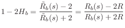
We conclude that ``in-phase vibrations'' see a longer effective string length, lengthened by the phase delay of
We similarly conclude that the ``anti-phase vibrations'' see no length correction at all, because the bridge point does not move at all in this case. In other words, any bridge termination at a point is rigid with respect to anti-phase vibration of the two strings connected to that point.
The above analysis predicts that, in ``stiffness controlled'' frequency intervals (in which the bridge ``looks like a damped spring''), the ``initial fast decay'' of a piano note should be a measurably flatter than the ``aftersound'' which should be exactly in tune as if the termination were rigid.
Next Section:
Digital Waveguide Mesh
Previous Section:
Loaded Waveguide Junctions