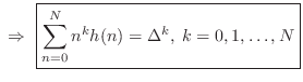
Lagrange Interpolation
Lagrange interpolation is a well known, classical technique for interpolation [193]. It is also called Waring-Lagrange interpolation, since Waring actually published it 16 years before Lagrange [309, p. 323]. More generically, the term polynomial interpolation normally refers to Lagrange interpolation. In the first-order case, it reduces to linear interpolation.
Given a set of ![]() known samples
known samples ![]() ,
,
![]() , the
problem is to find the unique order
, the
problem is to find the unique order ![]() polynomial
polynomial ![]() which
interpolates the samples.5.2The solution can be expressed as a linear combination of elementary
which
interpolates the samples.5.2The solution can be expressed as a linear combination of elementary
![]() th order polynomials:
th order polynomials:
where
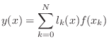
![$\displaystyle l_k(x_j) = \delta_{kj} \isdef \left\{\begin{array}{ll}
1, & j=k, \\ [5pt]
0, & j\neq k. \\
\end{array}\right.
$](http://www.dsprelated.com/josimages_new/pasp/img1008.png)
![\includegraphics[width=\twidth]{eps/lagrangebases}](http://www.dsprelated.com/josimages_new/pasp/img1011.png) |
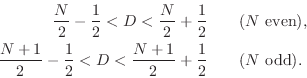
Interpolation of Uniformly Spaced Samples
In the uniformly sampled case (![]() for some sampling interval
for some sampling interval
![]() ), a Lagrange interpolator can be viewed as a Finite Impulse
Response (FIR) filter [449]. Such filters are often called
fractional delay filters
[267], since they are filters providing a non-integer time delay, in general.
Let
), a Lagrange interpolator can be viewed as a Finite Impulse
Response (FIR) filter [449]. Such filters are often called
fractional delay filters
[267], since they are filters providing a non-integer time delay, in general.
Let ![]() denote the impulse response of such a
fractional-delay filter. That is, assume the interpolation at point
denote the impulse response of such a
fractional-delay filter. That is, assume the interpolation at point
![]() is given by
is given by
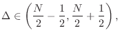
where we have set ![]() for simplicity, and used the fact that
for simplicity, and used the fact that
![]() for
for
![]() in the case of ``true
interpolators'' that pass through the given samples exactly. For best
results,
in the case of ``true
interpolators'' that pass through the given samples exactly. For best
results, ![]() should be evaluated in a one-sample range centered
about
should be evaluated in a one-sample range centered
about ![]() . For delays outside the central one-sample range, the
coefficients can be shifted to translate the desired delay into
that range.
. For delays outside the central one-sample range, the
coefficients can be shifted to translate the desired delay into
that range.
Fractional Delay Filters
In fractional-delay filtering applications, the interpolator typically slides forward through time to produce a time series of interpolated values, thereby implementing a non-integer signal delay:
The frequency response [449] of the fractional-delay
FIR filter ![]() is
is
Lagrange Interpolation Optimality
As derived in §4.2.14, Lagrange fractional-delay filters are maximally flat in the frequency domain at dc. That is,
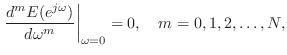
Figure 4.11 compares Lagrange and optimal Chebyshev fractional-delay
filter frequency responses. Optimality in the Chebyshev
sense means minimizing the worst-case
error over a given frequency band (in this case,
![]() ). While Chebyshev optimality is often the most desirable
choice, we do not have closed-form formulas for such solutions, so they
must be laboriously pre-calculated, tabulated, and interpolated to
produce variable-delay filtering [358].
). While Chebyshev optimality is often the most desirable
choice, we do not have closed-form formulas for such solutions, so they
must be laboriously pre-calculated, tabulated, and interpolated to
produce variable-delay filtering [358].
![\includegraphics[width=3.5in]{eps/lag}](http://www.dsprelated.com/josimages_new/pasp/img1030.png) |
Explicit Lagrange Coefficient Formulas
Given a desired fractional delay of ![]() samples, the Lagrange
fraction-delay impulse response can be written in closed form as
samples, the Lagrange
fraction-delay impulse response can be written in closed form as
The following table gives specific examples for orders 1, 2, and 3:
Lagrange Interpolation Coefficient Symmetry
As shown in [502, §3.3.3], directly substituting into
Eq.![]() (4.7) derives the following coefficient symmetry
property for the interpolation coefficients (impulse response) of a
Lagrange fractional delay filter:
(4.7) derives the following coefficient symmetry
property for the interpolation coefficients (impulse response) of a
Lagrange fractional delay filter:
where
Matlab Code for Lagrange Interpolation
A simple matlab function for computing the coefficients of a Lagrange fractional-delay FIR filter is as follows:
function h = lagrange( N, delay )

n = 0:N;
h = ones(1,N+1);
for k = 0:N
    index = find(n ~= k);
    h(index) = h(index) *  (delay-k)./ (n(index)-k);
end
Maxima Code for Lagrange Interpolation
The maxima program is free and open-source, like Octave for matlab:5.3
  (%i1) lagrange(N, n) :=
           product(if equal(k,n) then 1
                  else (D-k)/(n-k), k, 0, N);

  (%o1) lagrange(N, n) := product(if equal(k, n) then 1

                                       D - k
                                  else -----, k, 0, N)
                                       n - k
Usage examples in maxima:
  (%i2) lagrange(1,0);
  (%o2)                             1 - D

  (%i3) lagrange(1,1);
  (%o3)                               D

  (%i4) lagrange(4,0);
                           (1 - D) (D - 4) (D - 3) (D - 2)
  (%o4)                 - -------------------------------
                                         24
  (%i5) ratsimp(lagrange(4,0));
                           4       3       2
                          D  - 10 D  + 35 D  - 50 D + 24
  (%o5)                  ------------------------------
                                      24

  (%i6) expand(lagrange(4,0));
                            4      3       2
                           D    5 D    35 D    25 D
  (%o6)                    -- - ---- + ----- - ---- + 1
                           24    12     24      12

  (%i7) expand(lagrange(4,0)), numer;
                           4                     3
  (%o7) 0.041666666666667 D  - 0.41666666666667 D
                           2
      + 1.458333333333333 D  - 2.083333333333333 D + 1.0
Faust Code for Lagrange Interpolation
The Faust programming language for signal processing [453,450] includes support for Lagrange fractional-delay filtering, up to order five, in the library file filter.lib. For example, the fourth-order case is listed below:
// fourth-order (quartic) case, delay d in [1.5,2.5]
fdelay4(n,d,x) = delay(n,id,x)   * fdm1*fdm2*fdm3*fdm4/24
               + delay(n,id+1,x) * (0-fd*fdm2*fdm3*fdm4)/6
               + delay(n,id+2,x) * fd*fdm1*fdm3*fdm4/4
               + delay(n,id+3,x) * (0-fd*fdm1*fdm2*fdm4)/6
               + delay(n,id+4,x) * fd*fdm1*fdm2*fdm3/24
with {
  o = 1.49999;
  dmo = d - o; // assumed nonnegative
  id = int(dmo);
  fd = o + frac(dmo);
  fdm1 = fd-1;
  fdm2 = fd-2;
  fdm3 = fd-3;
  fdm4 = fd-4;
};
An example calling program is shown in Fig.4.12.
// tlagrange.dsp - test Lagrange interpolation in Faust

import("filter.lib");

N = 16; % Allocated delay-line length

% Compare various orders:
D = 5.4;
process = 1-1' <: fdelay1(N,D),
                  fdelay2(N,D),
                  fdelay3(N,D),
                  fdelay4(N,D),
                  fdelay5(N,D);
// To see results:
// [in a shell]:
//   faust2octave tlagrange.dsp
// [at the Octave command prompt]:
//   plot(db(fft(faustout,1024)(1:512,:)));

// Alternate example for testing a range of 4th-order cases
// (change name to "process" and rename "process" above):
process2  = 1-1' <: fdelay4(N, 1.5),
                    fdelay4(N, 1.6),
                    fdelay4(N, 1.7),
                    fdelay4(N, 1.8),
                    fdelay4(N, 1.9),
                    fdelay4(N, 2.0),
                    fdelay4(N, 2.1),
                    fdelay4(N, 2.2),
                    fdelay4(N, 2.3),
                    fdelay4(N, 2.4),
                    fdelay4(N, 2.499),
                    fdelay4(N, 2.5);
|
Lagrange Frequency Response Examples
The following examples were generated using Faust code similar to that in Fig.4.12 and the faust2octave command distributed with Faust.
Orders 1 to 5 on a fractional delay of 0.4 samples
Figure ![]() shows the
amplitude responses of Lagrange interpolation, orders 1 through 5, for
the case of implementing an interpolated delay line of length
shows the
amplitude responses of Lagrange interpolation, orders 1 through 5, for
the case of implementing an interpolated delay line of length ![]() samples. In all cases the interpolator follows a delay line of
appropriate length so that the interpolator coefficients operate over
their central one-sample interval.
Figure
samples. In all cases the interpolator follows a delay line of
appropriate length so that the interpolator coefficients operate over
their central one-sample interval.
Figure ![]() shows the
corresponding phase delays. As discussed in §4.2.10, the
amplitude response of every odd-order case is constrained to be zero at
half the sampling rate when the delay is half-way between integers,
which this example is near. As a result, the curves for the two
even-order interpolators lie above the three odd-order interpolators at
high frequencies in
Fig.
shows the
corresponding phase delays. As discussed in §4.2.10, the
amplitude response of every odd-order case is constrained to be zero at
half the sampling rate when the delay is half-way between integers,
which this example is near. As a result, the curves for the two
even-order interpolators lie above the three odd-order interpolators at
high frequencies in
Fig.![]() . It is
also interesting to note that the 4th-order interpolator, while showing
a wider ``pass band,'' exhibits more attenuation near half the sampling
rate than the 2nd-order interpolator.
. It is
also interesting to note that the 4th-order interpolator, while showing
a wider ``pass band,'' exhibits more attenuation near half the sampling
rate than the 2nd-order interpolator.
![\includegraphics[width=0.9\twidth]{eps/tlagrange-1-to-5-ar-c}](http://www.dsprelated.com/josimages_new/pasp/img1038.png) |
![\includegraphics[width=0.9\twidth]{eps/tlagrange-1-to-5-pd-c}](http://www.dsprelated.com/josimages_new/pasp/img1039.png) |
In the phase-delay plots of
Fig.![]() , all cases
are exact at frequency zero. At half the sampling rate
they all give 5 samples of delay.
, all cases
are exact at frequency zero. At half the sampling rate
they all give 5 samples of delay.
Note that all three odd-order phase delay curves look generally better
in Fig.![]() than
both of the even-order phase delays. Recall from
Fig.
than
both of the even-order phase delays. Recall from
Fig.![]() that the
two even-order amplitude responses outperformed all three odd-order
cases. This illustrates a basic trade-off between gain accuracy and
delay accuracy. The even-order interpolators show generally less
attenuation at high frequencies (because they are not constrained to
approach a gain of zero at half the sampling rate for a half-sample
delay), but they pay for that with a relatively inferior phase-delay
performance at high frequencies.
that the
two even-order amplitude responses outperformed all three odd-order
cases. This illustrates a basic trade-off between gain accuracy and
delay accuracy. The even-order interpolators show generally less
attenuation at high frequencies (because they are not constrained to
approach a gain of zero at half the sampling rate for a half-sample
delay), but they pay for that with a relatively inferior phase-delay
performance at high frequencies.
Order 4 over a range of fractional delays
Figures 4.15 and 4.16 show amplitude response and
phase delay, respectively, for 4th-order Lagrange interpolation
evaluated over a range of requested delays from ![]() to
to ![]() samples
in increments of
samples
in increments of ![]() samples. The amplitude response is ideal (flat
at 0 dB for all frequencies) when the requested delay is
samples. The amplitude response is ideal (flat
at 0 dB for all frequencies) when the requested delay is ![]() samples
(as it is for any integer delay), while there is maximum
high-frequency attenuation when the fractional delay is half a sample.
In general, the closer the requested delay is to an integer, the
flatter the amplitude response of the Lagrange interpolator.
samples
(as it is for any integer delay), while there is maximum
high-frequency attenuation when the fractional delay is half a sample.
In general, the closer the requested delay is to an integer, the
flatter the amplitude response of the Lagrange interpolator.
![\includegraphics[width=0.9\twidth]{eps/tlagrange-4-ar}](http://www.dsprelated.com/josimages_new/pasp/img1042.png) |
![\includegraphics[width=0.9\twidth]{eps/tlagrange-4-pd}](http://www.dsprelated.com/josimages_new/pasp/img1043.png) |
Note in Fig.4.16 how the phase-delay jumps
discontinuously, as a function of delay, when approaching the desired
delay of ![]() samples from below: The top curve in
Fig.4.16 corresponds to a requested delay of 2.5
samples, while the next curve below corresponds to 2.499 samples. The
two curves roughly coincide at low frequencies (being exact at dc),
but diverge to separate integer limits at half the sampling
rate. Thus, the ``capture range'' of the integer 2 at half the
sampling rate is numerically suggested to be the half-open interval
samples from below: The top curve in
Fig.4.16 corresponds to a requested delay of 2.5
samples, while the next curve below corresponds to 2.499 samples. The
two curves roughly coincide at low frequencies (being exact at dc),
but diverge to separate integer limits at half the sampling
rate. Thus, the ``capture range'' of the integer 2 at half the
sampling rate is numerically suggested to be the half-open interval
![]() .
.
Order 5 over a range of fractional delays
Figures 4.17 and 4.18 show amplitude response and
phase delay, respectively, for 5th-order Lagrange interpolation,
evaluated over a range of requested delays between ![]() and
and ![]() samples
in steps of
samples
in steps of ![]() samples. Note that the vertical scale in
Fig.4.17 spans
samples. Note that the vertical scale in
Fig.4.17 spans ![]() dB while that in
Fig.4.15 needed less than
dB while that in
Fig.4.15 needed less than ![]() dB, again due to the
constrained zero at half the sampling rate for odd-order interpolators
at the half-sample point.
dB, again due to the
constrained zero at half the sampling rate for odd-order interpolators
at the half-sample point.
![\includegraphics[width=0.9\twidth]{eps/tlagrange-5-ar}](http://www.dsprelated.com/josimages_new/pasp/img1047.png) |
![\includegraphics[width=0.9\twidth]{eps/tlagrange-5-pd}](http://www.dsprelated.com/josimages_new/pasp/img1048.png) |
Notice in Fig.4.18 how suddenly the phase-delay curves
near 2.5 samples delay jump to an integer number of samples as a
function of frequency near half the sample rate. The curve for
![]() samples swings down to 2 samples delay, while the curve for
samples swings down to 2 samples delay, while the curve for
![]() samples goes up to 3 samples delay at half the sample rate.
Since the gain is zero at half the sample rate when the requested
delay is
samples goes up to 3 samples delay at half the sample rate.
Since the gain is zero at half the sample rate when the requested
delay is ![]() samples, the phase delay may be considered to be
exactly
samples, the phase delay may be considered to be
exactly ![]() samples at all frequencies in that special case.
samples at all frequencies in that special case.
Avoiding Discontinuities When Changing Delay
We have seen examples (e.g., Figures 4.16 and 4.18)
of the general fact that every Lagrange interpolator provides an integer
delay at frequency
![]() , except when the interpolator gain
is zero at
, except when the interpolator gain
is zero at
![]() . This is true for any interpolator
implemented as a real FIR filter, i.e., as a linear combination of signal
samples using real coefficients.5.4Therefore, to avoid a relatively large discontinuity in phase delay (at
high frequencies) when varying the delay over time, the requested
interpolation delay should stay within a half-sample range of some fixed
integer, irrespective of interpolation order. This provides that the
requested delay stays within the ``capture zone'' of a single integer at
half the sampling rate. Of course, if the delay varies by more than one
sample, there is no way to avoid the high-frequency discontinuity in the
phase delay using Lagrange interpolation.
. This is true for any interpolator
implemented as a real FIR filter, i.e., as a linear combination of signal
samples using real coefficients.5.4Therefore, to avoid a relatively large discontinuity in phase delay (at
high frequencies) when varying the delay over time, the requested
interpolation delay should stay within a half-sample range of some fixed
integer, irrespective of interpolation order. This provides that the
requested delay stays within the ``capture zone'' of a single integer at
half the sampling rate. Of course, if the delay varies by more than one
sample, there is no way to avoid the high-frequency discontinuity in the
phase delay using Lagrange interpolation.
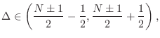
Even-order Lagrange interpolators have an integer at the midpoint of their central one-sample range, so they spontaneously offer a one-sample variable delay free of high-frequency discontinuities.
Odd-order Lagrange interpolators, on the other hand, must be shifted by
![]() sample in either direction in order to be centered about an
integer delay. This can result in stability problems if the
interpolator is used in a feedback loop, because the interpolation gain
can exceed 1 at some frequency when venturing outside the central
one-sample range (see §4.2.11 below).
sample in either direction in order to be centered about an
integer delay. This can result in stability problems if the
interpolator is used in a feedback loop, because the interpolation gain
can exceed 1 at some frequency when venturing outside the central
one-sample range (see §4.2.11 below).
In summary, discontinuity-free interpolation ranges include
Wider delay ranges, and delay ranges not centered about an integer
delay, will include a phase discontinuity in the delay response (as a
function of delay) which is largest at frequency
![]() , as
seen in Figures 4.16 and 4.18.
, as
seen in Figures 4.16 and 4.18.
Lagrange Frequency Response Magnitude Bound
The amplitude response of fractional delay filters based on Lagrange
interpolation is observed to be bounded by 1 when the desired delay
![]() lies within half a sample of the midpoint of the coefficient
span [502, p. 92], as was the case in all preceeding examples
above. Moreover, even-order interpolators are observed to have
this boundedness property over a two-sample range centered on the
coefficient-span midpoint [502, §3.3.6]. These assertions are
easily proved for orders 1 and 2. For higher orders, a general proof
appears not to be known, and the conjecture is based on numerical
examples. Unfortunately, it has been observed that the gain of some
odd-order Lagrange interpolators do exceed 1 at some frequencies when
used outside of their central one-sample range [502, §3.3.6].
lies within half a sample of the midpoint of the coefficient
span [502, p. 92], as was the case in all preceeding examples
above. Moreover, even-order interpolators are observed to have
this boundedness property over a two-sample range centered on the
coefficient-span midpoint [502, §3.3.6]. These assertions are
easily proved for orders 1 and 2. For higher orders, a general proof
appears not to be known, and the conjecture is based on numerical
examples. Unfortunately, it has been observed that the gain of some
odd-order Lagrange interpolators do exceed 1 at some frequencies when
used outside of their central one-sample range [502, §3.3.6].
Even-Order Lagrange Interpolation Summary
We may summarize some characteristics of even-order Lagrange fractional delay filtering as follows:
- Two-sample bounded-by-1 delay-range instead of only one-sample
- No gain zero at half the sampling rate for the middle delay
- No phase-delay discontinuity when crossing the middle delay
- Optimal (central) delay range is centered about an integer
Odd-Order Lagrange Interpolation Summary
In contrast to even-order Lagrange interpolation, the odd-order case has the following properties (in fractional delay filtering applications):
- Improved phase-delay accuracy at the expense of decreased
amplitude-response accuracy (low-order examples in
Fig.
![[*]](../icons/crossref.png) )
)
- Optimal (centered) delay range lies between two integers
To avoid a discontinuous phase-delay jump at high frequencies when crossing the middle delay, the delay range can be shifted to
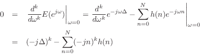
Proof of Maximum Flatness at DC
The maximumally flat fractional-delay FIR filter is obtained by equating
to zero all ![]() leading terms in the Taylor (Maclaurin) expansion of
the frequency-response error at dc:
leading terms in the Taylor (Maclaurin) expansion of
the frequency-response error at dc:
![\begin{eqnarray*}
\left\vert\left[p_i^{j-1}\right]\right\vert &=& \prod_{j>i}(p_...
...ts\\
&&(p_{N-1}-p_{N-2})(p_N-p_{N-2})\cdots\\
&&(p_N-p_{N-1}).
\end{eqnarray*}](http://www.dsprelated.com/josimages_new/pasp/img1065.png)
Making this substitution in the solution obtained by Cramer's rule
yields that the impulse response of the order ![]() , maximally flat,
fractional-delay FIR filter may be written in closed form as
, maximally flat,
fractional-delay FIR filter may be written in closed form as

Further details regarding the theory of Lagrange interpolation can be found (online) in [502, Ch. 3, Pt. 2, pp. 82-84].
Variable Filter Parametrizations
In practical applications of Lagrange Fractional-Delay Filtering
(LFDF), it is typically necessary to compute the FIR interpolation
coefficients
![]() as a function of the desired delay
as a function of the desired delay
![]() , which is usually time varying. Thus, LFDF is a special case
of FIR variable filtering in which the FIR coefficients must be
time-varying functions of a single delay parameter
, which is usually time varying. Thus, LFDF is a special case
of FIR variable filtering in which the FIR coefficients must be
time-varying functions of a single delay parameter ![]() .
.
Table Look-Up
A general approach to variable filtering is to tabulate the filter
coefficients as a function of the desired variables. In the case of
fractional delay filters, the impulse response
![]() is
tabulated as a function of delay
is
tabulated as a function of delay
![]() ,
,
![]() ,
,
![]() , where
, where ![]() is the
interpolation-filter order. For each
is the
interpolation-filter order. For each ![]() ,
, ![]() may be sampled
sufficiently densely so that linear interpolation will give a
sufficiently accurate ``interpolated table look-up'' of
may be sampled
sufficiently densely so that linear interpolation will give a
sufficiently accurate ``interpolated table look-up'' of
![]() for each
for each ![]() and (continuous)
and (continuous) ![]() . This method is commonly used
in closely related problem of sampling-rate conversion
[462].
. This method is commonly used
in closely related problem of sampling-rate conversion
[462].
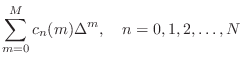
Polynomials in the Delay
A more parametric approach is to formulate each filter coefficient
![]() as a polynomial in the desired delay
as a polynomial in the desired delay ![]() :
:
Taking the z transform of this expression leads to the interesting and useful Farrow structure for variable FIR filters [134].
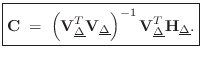
Farrow Structure
Taking the z transform of Eq.![]() (4.9) yields
(4.9) yields
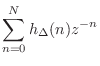
![$\displaystyle \sum_{n=0}^N \left[\sum_{m=0}^M c_n(m)\Delta^m\right]z^{-n}$](http://www.dsprelated.com/josimages_new/pasp/img1079.png)
![$\displaystyle \sum_{m=0}^M \left[\sum_{n=0}^N c_n(m) z^{-n}\right]\Delta^m$](http://www.dsprelated.com/josimages_new/pasp/img1080.png)
Since
Such a parametrization of a variable filter as a polynomial in
fixed filters ![]() is called a Farrow structure
[134,502]. When the polynomial Eq.
is called a Farrow structure
[134,502]. When the polynomial Eq.![]() (4.10) is
evaluated using Horner's rule,5.5 the efficient structure of
Fig.4.19 is obtained. Derivations of Farrow-structure
coefficients for Lagrange fractional-delay filtering are introduced in
[502, §3.3.7].
(4.10) is
evaluated using Horner's rule,5.5 the efficient structure of
Fig.4.19 is obtained. Derivations of Farrow-structure
coefficients for Lagrange fractional-delay filtering are introduced in
[502, §3.3.7].
![\includegraphics[width=\twidth]{eps/farrow}](http://www.dsprelated.com/josimages_new/pasp/img1087.png) |
As we will see in the next section, Lagrange interpolation can be
implemented exactly by the Farrow structure when ![]() . For
. For ![]() ,
approximations that do not satisfy the exact interpolation property
can be computed [148].
,
approximations that do not satisfy the exact interpolation property
can be computed [148].
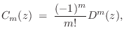
Farrow Structure Coefficients
Beginning with a restatement of Eq.![]() (4.9),
(4.9),

![$\displaystyle h_\Delta(n) \eqsp
\underbrace{%
\left[\begin{array}{ccccc} 1 & \...
...y}{c} C_n(0) \\ [2pt] C_n(1) \\ [2pt] \vdots \\ [2pt] C_n(M)\end{array}\right]
$](http://www.dsprelated.com/josimages_new/pasp/img1090.png)
![$\displaystyle \underbrace{\left[\begin{array}{cccc}h_\Delta(0)\!&\!h_\Delta(1)\...
...\vdots \\
C_0(M) & C_1(M) & \cdots & C_N(M)
\end{array}\right]}_{\mathbf{C}}
$](http://www.dsprelated.com/josimages_new/pasp/img1091.png)
where
![$\displaystyle \mathbf{H}_{\underline{\Delta}}\isdefs \left[\begin{array}{c} \un...
...elta_0}^T \\ [2pt] \vdots \\ [2pt] \underline{h}_{\Delta_L}^T\end{array}\right]$](http://www.dsprelated.com/josimages_new/pasp/img1095.png) and
and![$\displaystyle \qquad
\mathbf{V}_{\underline{\Delta}}\isdefs \left[\begin{array}...
...ta_0}^T \\ [2pt] \vdots \\ [2pt] \underline{V}_{\Delta_L}^T\end{array}\right].
$](http://www.dsprelated.com/josimages_new/pasp/img1096.png)
Differentiator Filter Bank
Since, in the time domain, a Taylor series expansion of
![]() about time
about time ![]() gives
gives
![\begin{eqnarray*}
x(n-\Delta)
&=& x(n) -\Delta\, x^\prime(n)
+ \frac{\Delta^2...
...D^2(z) + \cdots
+ \frac{(-\Delta)^k}{k!}D^k(z) + \cdots \right]
\end{eqnarray*}](http://www.dsprelated.com/josimages_new/pasp/img1101.png)
where ![]() denotes the transfer function of the ideal differentiator,
we see that the
denotes the transfer function of the ideal differentiator,
we see that the ![]() th filter in Eq.
th filter in Eq.![]() (4.10) should approach
(4.10) should approach
in the limit, as the number of terms
Farrow structures such as Fig.4.19 may be used to implement any
one-parameter filter variation in terms of several constant
filters. The same basic idea of polynomial expansion has been applied
also to time-varying filters (
![]() ).
).
Recent Developments in Lagrange Interpolation
Franck (2008) [148] provides a nice overview of the various structures being used for Lagrange interpolation, along with their computational complexities and depths (relevant to parallel processing). He moreover proposes a novel computation having linear complexity and log depth that is especially well suited for parallel processing architectures.
Relation of Lagrange to Sinc Interpolation
For an infinite number of equally spaced
samples, with spacing
![]() , the Lagrangian basis
polynomials converge to shifts of the sinc function, i.e.,
, the Lagrangian basis
polynomials converge to shifts of the sinc function, i.e.,
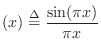
The equivalence of sinc interpolation to Lagrange interpolation was apparently first published by the mathematician Borel in 1899, and has been rediscovered many times since [309, p. 325].
A direct proof can be based on the equivalance between Lagrange
interpolation and windowed-sinc interpolation using a ``scaled
binomial window'' [262,502]. That is,
for a fractional sample delay of ![]() samples, multiply the
shifted-by-
samples, multiply the
shifted-by-![]() , sampled, sinc function
, sampled, sinc function
![$\displaystyle (n-D) = \frac{\sin[\pi(n-D)]}{\pi(n-D)}
$](http://www.dsprelated.com/josimages_new/pasp/img1113.png)
A more recent alternate proof appears in [557].
Next Section:
Thiran Allpass Interpolators
Previous Section:
Delay-Line Interpolation