




Fixed-Point Analysis of a PDM Modulator with GNU Octave's FXP Package
How to deploy fixed-point in a system-level model, and use it to find, measure, and fix quantization damage before it reaches RTL.
Introduction
This article walks through a small but complete case study: a first-order PDM modulator modeled in GNU Octave, first in double precision, then re-run through the same code with a genuine fixed-point data type substituted in. The tool that makes the substitution painless is "fxp", an Octave class (installable as a package, currently at v3.1.1) built specifically to model hardware fixed-point arithmetic.
The test case: a first-order PDM/ΔΣ loop
The model under test was taken over from [1], is a minimal first-order delta-sigma loop driving a single-bit quantizer, as shown in Fig. 1.
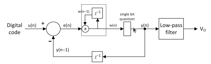
Fig. 1. First order delta-sigma modulator for pulse density modulation.
The modulator is modeled in the Octave function pdm_dsm (code attached in the appendix). The code implements the depicted schematic. The function checks whether to seed its internal states as plain doubles or as "fxp" objects carrying the same format as the input.
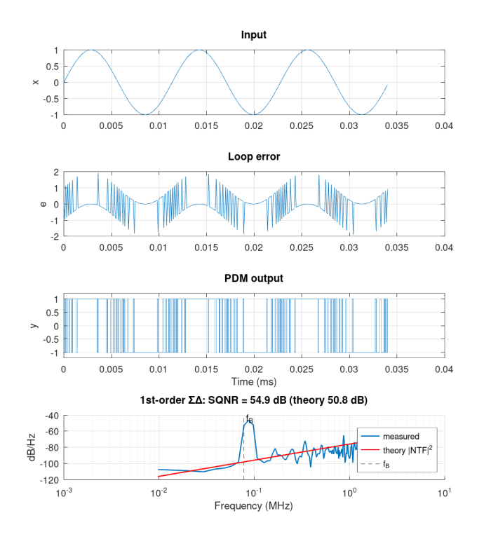
Fig. 2. First order delta-sigma modulator a) input sinusoidal signal x[n], b) loop error signal e[n], c) PDM output y[n], d) PSD of PDM signal.
Test Setup
A simple test setup has been constructed to test the functionality and behavior of the DSM loop and investigate the fixed-point impact and analysis on it. The design parameters for this setup is as follow: sampling frequency (fs=10MHz), single tone input frequency (fo=77.3kHz), over sampling ratio (OSR=64), input amplitude of 1 (full scale FS=2), number of sample (n=1024 for both time and frequency domains), Hann window for FFT analysis.
The test setup will examine the following fixed-point configurations:
|
Name |
S |
WL |
FL |
Range |
|---|---|---|---|---|
|
s6[0,5] |
1 |
6 |
5 |
[-1, 0.96875] |
|
s8[0,7] |
1 |
8 |
7 |
[-1, 0.9921875] |
|
s10[0,9] |
1 |
10 |
9 |
[-1, 0.998] |
|
s12[0,11] |
1 |
12 |
11 |
[-1, 0.9995] |
Run 01:
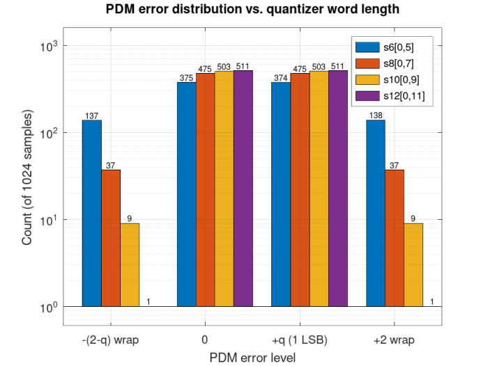
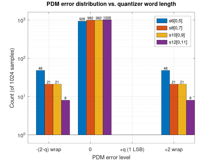
Baseline input amplitude A = 1 (full-scale, ±1.0 swing). PDM output error distribution across the four word-lengths, log-scale count of 1024 samples per configuration, with the exact count labeled above every bar.
Run 02:
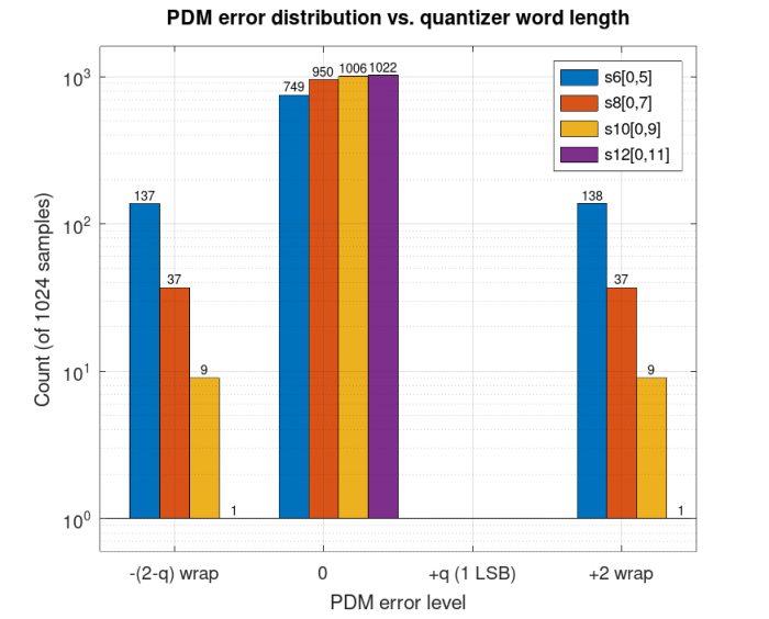
Same sweep, same A = 1 input, with one change: the internal "fxp" word carrying the loop state is extended by one integer bit (WL -> WL+1, FL unchanged) to remove any headroom-driven wrap at the top of the integrator.
Run 03:
Baseline internal word-lengths restored; instead, the input amplitude is halved to A = 0.5 (±0.5 swing instead of ±1.0), giving the loop more room to move before it meets the quantizer's limits.
Run 04:
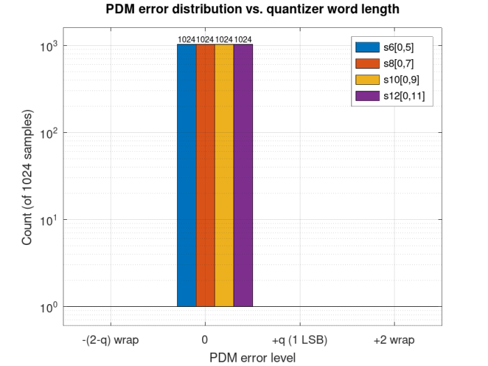
Here the floating-point loop is simulated with the same fixed-point-quantized input the "fxp" run uses, instead of the original, unquantized double — so both loops start from bit-identical samples.
Findings:
| Run | Findings |
| Run 01 | More bits make quantization error smaller |
| Run 02 | Internal bit-width growth is mandatory to accomodate for internal overflows |
| Run 03 | Reducing the input signal range moved the bars but not all in the same direction |
| Run 04 | Now it can be used as a golden reference for bit-true/cycle-true simulations (after removing false errors) |
Takeaways:
Quantization is real, but not every symptom that looks like quantization noise is quantization noise. The "fxp" class doesn't remove either kind of problem — nothing can — but it makes both visible, cheaply, in the same Octave model you already trust, before a single line of RTL is written.
That is the whole case for modeling fixed-point at the system level: not to predict a perfect number, but to know exactly where, how often, and why the finite word-length bites — and to know when it isn't the word-length at all — so every decision is measured rather than assumed.
References:
[1] V. Viegas, "Digital Pulse-Width and Pulse-Density Modulator Based on Binary Counting," 2025.
[2] https://github.com/ahmedshahein/pkg-fxp
[3] https://en.wikipedia.org/wiki/Pulse-density_modulation
Appendix:
DSM Model:
function [pdm, q_err, loop_err, intg_oup] = pdm_dsm(x)
  if isa(x, "fxp")
    n = length(x.vfxp);
    pdm   = fxp(zeros(1, n), x.S, x.WL+1, x.FL, 'ovf_action', x.ovf_action);
    err   = fxp(zeros(1, n), x.S, x.WL+1, x.FL, 'ovf_action', x.ovf_action);
    wv    = fxp(zeros(1, n), x.S, x.WL+1, x.FL, 'ovf_action', x.ovf_action);
    y_dly = fxp(0, x.S, x.WL+1, x.FL, 'ovf_action', x.ovf_action);
    w_dly = fxp(0, x.S, x.WL+1, x.FL, 'ovf_action', x.ovf_action);
  else
    n   = length(x);
    pdm   = zeros(1, n);
    err   = zeros(1, n);
    wv    = zeros(1, n);
    y_dly = 0;
    w_dly = 0;
  end

  for i = 1:n
    e       = x(i) - y_dly;                 % loop error
    w       = e + w_dly;                    % integrator
    y       = single_bit_quantizer(w);      % single-bit quantizer
    y_dly   = y;
    w_dly   = w;
    pdm(i)  = y;
    err(i)  = e;
    wv(i)   = w;
  end
  q = pdm - wv;                             % quantization error
  %% Assign outputs
  q_err     = q;    % quantization error
  loop_err  = err;  % loop error
  intg_oup  = wv;   % integrator state
Quantizer:
function q = single_bit_quantizer(x)
  if isa(x, "fxp")
    z = fxp(0, x.S, x.WL, x.FL, 'ovf_action', x.ovf_action);
    q = fxp(0, x.S, x.WL, x.FL, 'ovf_action', x.ovf_action);
  else
    z = 0;
  end
  for i = 1 : length(x)
    if (x(i) >= z)
      q(i) =  1;
    else
      q(i) = -1;
    end
  end
Test Script:
% ------------------------------------------------------------------------------
% Copyright (C) 2026 Ahmed Shahein
% ------------------------------------------------------------------------------
%
% ------------------------------------------------------------------------------
close all
clear
clc
%% Path for local helping functions
addpath('./funcs');
%% Design Parameters
fs    = 10e6;        % Sampling frequency (Hz)
n     = 2^10;        % Number of samples (2^10 leaves only 8 in-band bins)
nfft  = n;           % Number of FFT bins
OSR   = 64;          % Oversampling ratio
A     = 1;           % Input amplitude (quantizer levels are +/-1)
Delta = 2;           % Quantizer step: 2 for +/-1 levels, 1 for {0,1}
L     = 1;           % Modulator order (for theory)
nharm = 5;           % Harmonics excluded for SNR
fB    = fs/(2*OSR);  % Signal band edge (78.125 kHz)
df    = fs/nfft;     % Bin width (152.6 Hz)
win_type = 'hann';   % 'hann' | 'blackmanharris' | 'rect'
%% Coherent input tone: snap the wanted frequency to an odd bin
fo_req = 77.3e3;                    % requested tone frequency (Hz)
k      = round(fo_req/df);
k      = k + (mod(k,2) == 0);       % odd bin -> no repeated codes pattern
fo     = k*df;                      % actual tone frequency (Hz)
%% Input Stimuli
x = A*sin(2*pi*fo*(0:n-1)/fs);
inp_s  = 1;
inp_wl = [6,8,10,12];
inp_fl = [5,7,9,11];
fxp_tp = length(inp_wl);
for i = 1 : fxp_tp
  % Quantize input stimuli
  tmp = fxp(x, inp_s, inp_wl(i), inp_fl(i), 'ovf_action', 'sat');
  x = tmp.vfxp;
end

%% First-order SDM outputs
[pdm, q_err, loop_err, intg_oup] = pdm_dsm(x);
%% Fixed-point quantization configurations
##WL ≥ (SQNR_target - 1.76 - 10*log10(OSR)) / 6.02

%% Plot 3 cycles only
t     = (0:n-1)/fs;
nshow = min(n, round(3*fs/fo));     % three input periods
%% Fixed-point loop
for i = 1 : fxp_tp
  % Quantize input stimuli
  x_fxp = fxp(x, inp_s, inp_wl(i)+1, inp_fl(i), 'ovf_action', 'sat');
  % Perform sigma-delta modulation
  [pdm_fxp, q_err_fxp, loop_err_fxp, intg_oup_fxp] = pdm_dsm(x_fxp);
  % Input quantization error
  x_err(i,:) = x - x_fxp.vfxp;
  % Output quantization error
  pdm_err(i,:) = pdm-pdm_fxp.vfxp;
  % Frequency Domain Analysis
  [P, fb, S]      = psd_onesided(pdm_fxp.vfxp, fs, win_type);
  [SQNR_dB, Ps]   = calc_sqnr(P, S, fo, fB);
  T               = sdm_theory(A, Delta, OSR, L);
  % Plotting
  names = {'s6','s8','s10','s12'};
  figure('name', names{i}, 'numbertitle', 'off');
  % Time-domain for input
  subplot(4,1,1)
  plot(t(1:nshow)*1e3, x_fxp(1:nshow).vfxp); grid on
  ylabel('x'); title('Input')
  % Time-domain for loop error
  subplot(4,1,2)
  plot(t(1:nshow)*1e3, loop_err_fxp(1:nshow).vfxp); grid on
  ylabel('e'); title('Loop error')
  % Time-domain for SDM output
  subplot(4,1,3)
  stairs(t(1:nshow)*1e3, pdm_fxp(1:nshow).vfxp); grid on; ylim([-1.2 1.2])
  ylabel('y'); xlabel('Time (ms)'); title('PDM output')
  % Frequency-domain for output
  subplot(4,1,4)
  psd_t = T.Pq*2/fs * abs(2*sin(pi*fb/fs)).^(2*L);   % theoretical shaped PSD
  plot_psd(fb, P, 'ENBW', S.enbw, 'df', df, ...
           'Theory', psd_t, ...
           'Labels', 'measured', 'TheoryLabels', 'theory |NTF|^2', ...
           'BandEdge', fB, ...
           'Title', sprintf('1st-order \\Sigma\\Delta: SQNR = %.1f dB (theory %.1f dB)', ...
                            SQNR_dB, T.SQNR_dB));
end
%% Error histogram plot
csvwrite('pdm_err.csv', pdm_err);
figure('name', 'hist', 'numbertitle', 'off');
X = 2*ones(size(pdm_err));                       % 0
X(pdm_err < -1)                = 1;              % -(2-q)
X(pdm_err > 0 & pdm_err < 1)   = 3;              % +q
X(pdm_err > 1)                 = 4;              % +2

hist(X', 1:fxp_tp);
p = findobj(gca, 'type', 'patch');
for k = 1:numel(p)
  v = get(p(k), 'vertices');
  v(v(:,2) == 0, 2) = 0.5;
  set(p(k), 'vertices', v);
end

n = zeros(4,4);
for i = 1:4, n(i,:) = hist(X(i,:), 1:4); end

set(gca, 'xtick', 1:4, 'xticklabel', {'-2+q', '0', '+q', '+2'});

legend('s6[0,5], q=2^{-5}', 's8[0,7], q=2^{-7}', ...
       's10[0,9], q=2^{-9}', 's12[0,11], q=2^{-11}');
% ------------------------------------------------------------------------------
% EOF
% ------------------------------------------------------------------------------- Comments
- Write a Comment Select to add a comment

Very nice write up Ahmed! Thanks for submitting this.
For those using Python, I like the fpbinary library for fixed-point modeling and analysis.

Appreciate your kind feedback Dan
Will definitely try the Python package, I believe I have tried the fxpmath before.
Regards,
Ahmed
To post reply to a comment, click on the 'reply' button attached to each comment. To post a new comment (not a reply to a comment) check out the 'Write a Comment' tab at the top of the comments.
Please login (on the right) if you already have an account on this platform.
Otherwise, please use this form to register (free) an join one of the largest online community for Electrical/Embedded/DSP/FPGA/ML engineers: