Non-Cylindrical Acoustic Tubes
In many situations, the wave impedance of the medium varies in a continuous manner rather than in discrete steps. This occurs, for example, in conical bores and flaring horns. In this section, based on [436], we will consider non-cylindrical acoustic tubes.
Horns as Waveguides
Waves in a horn can be analyzed as one-parameter waves, meaning that it is assumed that a constant-phase wavefront progresses uniformly along the horn. Each ``surface of constant phase'' composing the traveling wave has tangent planes normal to the horn axis and to the horn boundary. For cylindrical tubes, the surfaces of constant phase are planar, while for conical tubes, they are spherical [357,317,144]. The key property of a ``horn'' is that a traveling wave can propagate from one end to the other with negligible ``backscattering'' of the wave. Rather, it is smoothly ``guided'' from one end to the other. This is the meaning of saying that a horn is a ``waveguide''. The absence of backscattering means that the entire propagation path may be simulated using a pure delay line, which is very efficient computationally. Any losses, dispersion, or amplitude change due to horn radius variation (``spreading loss'') can be implemented where the wave exits the delay line to interact with other components.
Overview of Methods
We will first consider the elementary case of a conical acoustic tube. All smooth horns reduce to the conical case over sufficiently short distances, and the use of many conical sections, connected via scattering junctions, is often used to model an arbitrary bore shape [71]. The conical case is also important because it is essentially the most general shape in which there are exact traveling-wave solutions (spherical waves) [357].
Beyond conical bore shapes, however, one can use a Sturm-Liouville formulation to solve for one-parameter-wave scattering parameters [50]. In this formulation, the curvature of the bore's cross-section (more precisely, the curvature of the one-parameter wave's constant-phase surface area) is treated as a potential function that varies along the horn axis, and the solution is an eigenfunction of this potential. Sturm-Liouville analysis is well known in quantum mechanics for solving elastic scattering problems and for finding the wave functions (at various energy levels) for an electron in a nonuniform potential well.
When the one-parameter-wave assumption breaks down, and multiple acoustic modes are excited, the boundary element method (BEM) is an effective tool [190]. The BEM computes the acoustic field from velocity data along any enclosing surface. There also exist numerical methods for simulating wave propagation in varying cross-sections that include ``mode conversion'' [336,13,117].
This section will be henceforth concerned with non-cylindrical tubes in which backscatter and mode-conversion can be neglected, as treated in [317]. The only exact case is the cone, but smoothly varying horn shapes can be modeled approximately in this way.
Back to the Cone
Note that the cylindrical tube is a limiting case of a cone with its apex at infinity. Correspondingly, a plane wave is a limiting case of a spherical wave having infinite radius.
On a fundamental level, all pressure waves in 3D space are composed of spherical waves [357]. You may have learned about the Huygens-Fresnel principle in a physics class when it covered waves [295]. The Huygens-Fresnel principle states that the propagation of any wavefront can be modeled as the superposition of spherical waves emanating from all points along the wavefront [122, page 344]. This principle is especially valuable for intuitively understanding diffraction and related phenomena such as mode conversion (which happens, for example, when a plane wave in a horn hits a sharp bend or obstruction and breaks up into other kinds of waves in the horn).
Conical Acoustic Tubes
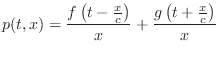
The conical acoustic tube is a one-dimensional waveguide which propagates circular sections of spherical pressure waves in place of the plane wave which traverses a cylindrical acoustic tube [22,349]. The wave equation in the spherically symmetric case is given by
where
Spherical coordinates are appropriate because simple closed-form
solutions to the wave equation are only possible when the forced boundary
conditions lie along coordinate planes. In the case of a cone, the
boundary conditions lie along a conical section of a sphere. It can be
seen that the wave equation in a cone is identical to the wave equation in
a cylinder, except that ![]() is replaced by
is replaced by ![]() . Thus, the solution is a
superposition of left- and right-going traveling wave components, scaled by
. Thus, the solution is a
superposition of left- and right-going traveling wave components, scaled by
![]() :
:
where
In cylindrical tubes, the velocity wave is in phase with the pressure wave. This is not the case with conical or more general tubes. The velocity of a traveling may be computed from the corresponding traveling pressure wave by dividing by the wave impedance.
Digital Simulation
A discrete-time simulation of the above solution may be obtained by simply
sampling the traveling-wave amplitude at intervals of ![]() seconds, which implies a spatial sampling interval of
seconds, which implies a spatial sampling interval of
![]() meters. Sampling is carried out mathematically by the
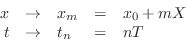
change of variables
meters. Sampling is carried out mathematically by the
change of variables
![\begin{eqnarray*}
x_mp(t_n,x_m) &\,\mathrel{\mathop=}\,& f(t_n- x_m/c)+g(t_n+ x...
...hop=}\,& f\left[(n-m)T-x_0/c\right]+ g\left[(n+m)T+x_0/c\right].
\end{eqnarray*}](http://www.dsprelated.com/josimages_new/pasp/img4258.png)
Define
![\includegraphics[width=\twidth]{eps/fcideal}](http://www.dsprelated.com/josimages_new/pasp/img4261.png) |
A more compact simulation diagram which stands for either sampled or continuous simulation is shown in Figure C.44. The figure emphasizes that the ideal, lossless waveguide is simulated by a bidirectional delay line.
![\includegraphics[width=\twidth]{eps/fcone}](http://www.dsprelated.com/josimages_new/pasp/img4262.png)
As in the case of uniform waveguides, the digital simulation of the traveling-wave solution to the lossless wave equation in spherical coordinates is exact at the sampling instants, to within numerical precision, provided that the traveling waveshapes are initially bandlimited to less than half the sampling frequency. Also as before, bandlimited interpolation can be used to provide time samples or position samples at points off the simulation grid. Extensions to include losses, such as air absorption and thermal conduction, or dispersion, can be carried out as described in §2.3 and §C.5 for plane-wave propagation (through a uniform wave impedance).
The simulation of Fig.C.44 suffices to simulate an isolated conical frustum, but what if we wish to interconnect two or more conical bores? Even more importantly, what driving-point impedance does a mouthpiece ``see'' when attached to the narrow end of a conical bore? The preceding only considered pressure-wave behavior. We must now also find the velocity wave, and form their ratio to obtain the driving-point impedance of a conical tube.
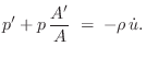
Momentum Conservation in Nonuniform Tubes
Newton's second law ``force equals mass times acceleration'' implies that
the pressure gradient in a gas is proportional to the acceleration of a
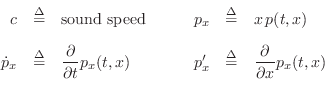
differential volume element in the gas. Let ![]() denote the area of the
surface of constant phase at radial coordinate
denote the area of the
surface of constant phase at radial coordinate ![]() in the tube. Then the
total force acting on the surface due to pressure is
in the tube. Then the
total force acting on the surface due to pressure is
![]() , as
shown in Fig.C.45.
, as
shown in Fig.C.45.
![\includegraphics[width=3in]{eps/fconic}](http://www.dsprelated.com/josimages_new/pasp/img4265.png)
The net force ![]() to the right across the volume element
between
to the right across the volume element
between ![]() and
and ![]() is then
is then
where, when time and/or position arguments have been dropped, as in the last line above, they are all understood to be
![\begin{eqnarray*}
dM(t,x) &=& \int_x^{x+dx} \rho(t,\xi) A(\xi)\,d\xi \\ [5pt]
&\...
...\rho A' \right)\frac{(dx)^2}{2}\\ [5pt]
&\approx& \rho\, A\,dx,
\end{eqnarray*}](http://www.dsprelated.com/josimages_new/pasp/img4273.png)
where ![]() denotes air density.
denotes air density.
The center-of-mass acceleration of the volume element can be written
as
![]() where
where ![]() is particle velocity.C.16 Applying Newton's second law
is particle velocity.C.16 Applying Newton's second law
![]() , we
obtain
, we
obtain
or, dividing through by
In terms of the logarithmic derivative of
Note that
Cylindrical Tubes
In the case of cylindrical tubes, the logarithmic derivative of the
area variation,
ln![]() , is zero, and Eq.
, is zero, and Eq.![]() (C.148)
reduces to the usual momentum conservation equation
(C.148)
reduces to the usual momentum conservation equation
![]() encountered when deriving the wave equation for plane waves
[318,349,47]. The present case reduces to the
cylindrical case when
encountered when deriving the wave equation for plane waves
[318,349,47]. The present case reduces to the
cylindrical case when

If we look at sinusoidal spatial waves,
![]() and
and
![]() , then
, then
![]() and
and
![]() , and the condition
for cylindrical-wave behavior becomes
, and the condition
for cylindrical-wave behavior becomes
![]() , i.e., the spatial
frequency of the wall variation must be much less than that of the
wave. Another way to say this is that the wall must be approximately
flat across a wavelength. This is true for smooth horns/bores at
sufficiently high wave frequencies.
, i.e., the spatial
frequency of the wall variation must be much less than that of the
wave. Another way to say this is that the wall must be approximately
flat across a wavelength. This is true for smooth horns/bores at
sufficiently high wave frequencies.
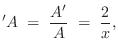
Wave Impedance in a Cone
From Eq.![]() (C.146) we have that the traveling-wave solution of the
wave equation in spherical coordinates can be expressed as
(C.146) we have that the traveling-wave solution of the
wave equation in spherical coordinates can be expressed as
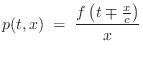
i.e., it can be expressed in terms of its own time derivative. This is a general property of any traveling wave.
![\includegraphics[width=\twidth]{eps/fconeparams}](http://www.dsprelated.com/josimages_new/pasp/img4294.png)
Referring to Fig.C.46, the area function ![]() can be
written for any cone in terms of the distance from its apex as
can be
written for any cone in terms of the distance from its apex as
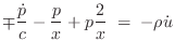
Substituting the logarithmic derivative of ![]() and
and ![]() from
Eq.
from
Eq.![]() (C.150) into the momentum-conservation equation
Eq. (C.148) yields
(C.150) into the momentum-conservation equation
Eq. (C.148) yields
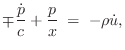
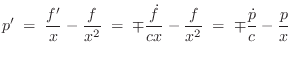
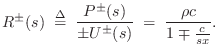
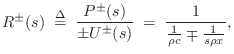
We can now solve for the wave impedance in each direction, where
the wave impedance may be defined (§7.1)
as the Laplace transform of the traveling pressure divided by
the Laplace transform of the corresponding traveling velocity wave:
 |
|||
 |
We introduce the shorthand
Note that for a cylindrical tube, the wave impedance in both directions is
![]() , and there is no frequency dependence. A wavelength
or more away from the conical tip, i.e., for
, and there is no frequency dependence. A wavelength
or more away from the conical tip, i.e., for
![]() ,
where
,
where ![]() is the spatial wavelength, the wave impedance again approaches
that of a cylindrical bore. However, in conical musical instruments,
the fundamental wavelength is typically twice the bore length, so the
complex nature of the wave impedance is important throughout the bore and
approaches being purely imaginary near the mouthpiece. This is
especially relevant to conical-bore double-reeds, such as the bassoon.
is the spatial wavelength, the wave impedance again approaches
that of a cylindrical bore. However, in conical musical instruments,
the fundamental wavelength is typically twice the bore length, so the
complex nature of the wave impedance is important throughout the bore and
approaches being purely imaginary near the mouthpiece. This is
especially relevant to conical-bore double-reeds, such as the bassoon.
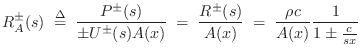
Writing the wave impedance as
Up to now, we have been defining wave impedance as pressure divided by particle velocity. In acoustic tubes, volume velocity is what is conserved at a junction between two different acoustic tube types. Therefore, in acoustic tubes, we define the wave impedance as the ratio of pressure to volume velocity
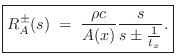
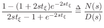
This is the wave impedance we use to compute the generalized reflection and transmission coefficients at a change in cross-sectional area and/or taper angle in a conical acoustic tube. Note that it has a zero at
In this case, the equivalent mass is
![]() . It would perhaps be more satisfying if the equivalent mass in
the conical wave impedance were instead
. It would perhaps be more satisfying if the equivalent mass in
the conical wave impedance were instead
![]() which is the
mass of air contained in a cylinder of radius
which is the
mass of air contained in a cylinder of radius ![]() projected back to
the tip of the cone. However, the ``acoustic mass'' cannot be
physically equivalent to mechanical mass. To see this, consider that
the impedance of a mechanical mass is
projected back to
the tip of the cone. However, the ``acoustic mass'' cannot be
physically equivalent to mechanical mass. To see this, consider that
the impedance of a mechanical mass is ![]() which is in physical units
of mass per unit time, and by definition of mechanical impedance this
equals force over velocity. The impedance in an acoustic tube, on the
other hand, must be in units of pressure (force/area) divided by
volume velocity (velocity
which is in physical units
of mass per unit time, and by definition of mechanical impedance this
equals force over velocity. The impedance in an acoustic tube, on the
other hand, must be in units of pressure (force/area) divided by
volume velocity (velocity ![]() area) and this reduces to
area) and this reduces to
The real part of the wave impedance corresponds to transportation of wave
energy, the imaginary part is a so-called ``reactance'' and does not
correspond to power transfer. Instead, it corresponds to a ``standing
wave'' which is created by equal and opposite power flow, or an
``evanescent wave'' (§C.8.2), which is a non-propagating,
exponentially decaying, limiting form of a traveling wave in which the
``propagation constant'' is purely imaginary due to being at a
frequency above or below a ``cut off'' frequency for the waveguide
[295,122]. Driving an ideal mass at the end of a
waveguide results in total reflection of all incident wave energy
along with a quarter-cycle phase shift. Another interpretation is
that the traveling wave becomes a standing wave at the tip of the
cone. This is one way to see how the resonances of a cone can be the
same as those of a cylinder the same length which is open on
both ends. (One might first expect the cone to behave like a
cylinder which is open on one end and closed on the other.) Because
the impedance approaches a purely imaginary zero at the tip, it looks
like a mass (with impedance
![]() ). The ``piston of air'' at
the open end similarly looks like a mass
[285].
). The ``piston of air'' at
the open end similarly looks like a mass
[285].
More General One-Parameter Waves
The wave impedance derivation above made use of known properties of waves
in cones to arrive at the wave impedances in the two directions of travel
in cones. We now consider how this solution might be generalized to
arbitrary bore shapes. The momentum conservation equation is already
applicable to any wavefront area variation ![]() :
:
Defining the spatially instantaneous phase velocity as
This reduces to the simple case of the uniform waveguide when the logarithmic derivative of cross-sectional area
Generalized Wave Impedance
Figure C.47 depicts a section of a conical bore which widens to the right connected to a section which narrows to the right. In addition, the cross-sectional areas are not matched at the junction.
The horizontal ![]() axis (taken along the boundary of the
cone) is chosen so that
axis (taken along the boundary of the
cone) is chosen so that ![]() corresponds to the apex of the cone. Let
corresponds to the apex of the cone. Let
![]() denote the cross-sectional area of the bore.
denote the cross-sectional area of the bore.
![\includegraphics[width=\twidth]{eps/fconecone}](http://www.dsprelated.com/josimages_new/pasp/img4350.png)
Since a piecewise-cylindrical approximation to a general acoustic tube can be regarded as a ``zeroth-order hold'' approximation. A piecewise conical approximation then uses first-order (linear) segments. One might expect that quadratic, cubic, etc., would give better and better approximations. However, such a power series expansion has a problem: In zero-order sections (cylinders), plane waves propagate as traveling waves. In first-order sections (conical sections), spherical waves propagate as traveling waves. However, there are no traveling wave types for higher-order waveguide flare (e.g., quadratic or higher) [357].
Since the digital waveguide model for a conic section is no more expensive to implement than that for a cylindrical section, (both are simply bidirectional delay lines), it would seem that modeling accuracy can be greatly improved for non-cylindrical bores (or parts of bores such as the bell) essentially for free. However, while the conic section itself costs nothing extra to implement, the scattering junctions between adjoining cone segments are more expensive computationally than those connecting cylindrical segments. However, the extra expense can be small. Instead of a single, real, reflection coefficient occurring at the interface between two cylinders of differing diameter, we obtain a first-order reflection filter at the interface between two cone sections of differing taper angle, as seen in the next section.
Generalized Scattering Coefficients
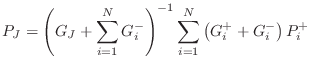
Generalizing the scattering coefficients at a multi-tube intersection
(§C.12) by replacing the usual real tube wave impedance
![]() by the complex generalized wave impedance
by the complex generalized wave impedance
Cylinder with Conical Cap
Consider a cylindrical acoustic tube adjoined to a converging conical cap, as depicted in Figure C.48a. We may consider the cylinder to be either open or closed on the left side, but everywhere else it is closed. Since such a physical system is obviously passive, an interesting test of acoustic theory is to check whether theory predicts passivity in this case.
![\includegraphics[scale=0.9]{eps/cylconesp}](http://www.dsprelated.com/josimages_new/pasp/img4359.png) |
It is well known that a growing exponential appears at the junction of two conical waveguides when the waves in one conical taper angle reflect from a section with a smaller (or more negative) taper angle [7,300,8,160,9]. The most natural way to model a growing exponential in discrete time is to use an unstable one-pole filter [506]. Since unstable filters do not normally correspond to passive systems, we might at first expect passivity to not be predicted. However, it turns out that all unstable poles are ultimately canceled, and the model is stable after all, as we will see. Unfortunately, as is well known in the field of automatic control, it is not practical to attempt to cancel an unstable pole in a real system, even when it is digital. This is because round-off errors will grow exponentially in the unstable feedback loop and eventually dominate the output.
The need for an unstable filter to model reflection and transmission at a converging conical junction has precluded the use of a straightforward recursive filter model [406]. Using special ``truncated infinite impulse response'' (TIIR) digital filters [540], an unstable recursive filter model can in fact be used in practice [528]. All that is then required is that the infinite-precision system be passive, and this is what we will show in the special case of Fig.C.48.
Scattering Filters at the Cylinder-Cone Junction
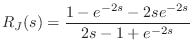
As derived in §C.18.4, the wave impedance (for volume velocity)
at frequency ![]() rad/sec in a converging cone is given by
rad/sec in a converging cone is given by
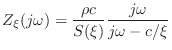 |
(C.152) |
where
(where
The reflectance and transmittance from the right of the junction are the same when there is no wavefront area discontinuity at the junction [300]. Both
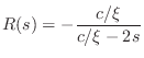
Reflectance of the Conical Cap
Let
![]() denote the time to propagate across the length of
the cone in one direction. As is well known [22], the reflectance
at the tip of an infinite cone is
denote the time to propagate across the length of
the cone in one direction. As is well known [22], the reflectance
at the tip of an infinite cone is ![]() for pressure waves. I.e., it
reflects like an open-ended cylinder. We ignore any absorption losses
propagating in the cone, so that the transfer function from the entrance of
the cone to the tip is
for pressure waves. I.e., it
reflects like an open-ended cylinder. We ignore any absorption losses
propagating in the cone, so that the transfer function from the entrance of
the cone to the tip is
![]() . Similarly, the transfer function from
the conical tip back to the entrance is also
. Similarly, the transfer function from
the conical tip back to the entrance is also
![]() . The complete
reflection transfer function from the entrance to the tip and back is then
. The complete
reflection transfer function from the entrance to the tip and back is then
| (C.155) |
Note that this is the reflectance a distance
We now want to interface the conical cap reflectance
![]() to the
cylinder. Since this entails a change in taper angle, there will be
reflection and transmission filtering at the cylinder-cone junction given
by Eq.
to the
cylinder. Since this entails a change in taper angle, there will be
reflection and transmission filtering at the cylinder-cone junction given
by Eq.![]() (C.154) and Eq.
(C.154) and Eq.![]() (C.155).
(C.155).
From inside the cylinder, immediately next to the cylinder-cone
junction shown in Fig.C.48, the reflectance of the conical cap is
readily derived from Fig.C.48b and Equations (C.154) and
(C.155) to be
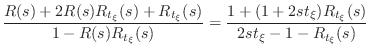 |
|||
 |
(C.156) |
where
| (C.157) |
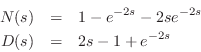
is the numerator of the conical cap reflectance, and
| (C.158) |
is the denominator. Note that for very large
Stability Proof
A transfer function
![]() is stable if there are no poles in
the right-half
is stable if there are no poles in
the right-half ![]() plane. That is, for each zero
plane. That is, for each zero ![]() of
of ![]() , we must
have
re
, we must
have
re![]() . If this can be shown, along with
. If this can be shown, along with
![]() , then the reflectance
, then the reflectance ![]() is shown to be
passive. We must also study the system zeros (roots of
is shown to be
passive. We must also study the system zeros (roots of ![]() ) in order to
determine if there are any pole-zero cancellations (common factors in
) in order to
determine if there are any pole-zero cancellations (common factors in
![]() and
and ![]() ).
).
Since
re![]() if and only if
re
if and only if
re![]() , for
, for
![]() , we may set
, we may set
![]() without loss of generality. Thus, we need only
study the roots of
without loss of generality. Thus, we need only
study the roots of
If this system is stable, we have stability also for all
![]() .
Since
.
Since ![]() is not a rational function of
is not a rational function of ![]() , the reflectance
, the reflectance ![]() may have infinitely many poles and zeros.
may have infinitely many poles and zeros.
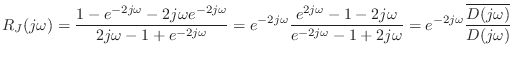
Let's first consider the roots of the denominator
| (C.159) |
At any solution

To obtain separate equations for the real and imaginary parts, set
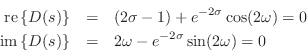
Both of these equations must hold at any pole of the reflectance. For
stability, we further require
![]() . Defining
. Defining
![]() and
and
![]() , we obtain the somewhat simpler conditions
, we obtain the somewhat simpler conditions
For any poles of ![]() on the
on the ![]() axis, we have
axis, we have ![]() , and
Eq.
, and
Eq.![]() (C.163) reduces to
(C.163) reduces to
It is well known that the ``sinc function''
We have so far proved that any poles on the ![]() axis must be at
axis must be at
![]() .
.
The same argument can be extended to the entire right-half
plane as follows. Going back to the more general case of
Eq.![]() (C.163), we have
(C.163), we have
 |
(C.164) |
Since
In the left-half plane, there are many potential poles.
Equation (C.162) has infinitely many solutions for each ![]() since the elementary inequality
since the elementary inequality
![]() implies
implies
![]() . Also, Eq.
. Also, Eq.![]() (C.163) has an increasing
number of solutions as
(C.163) has an increasing
number of solutions as ![]() grows more and more negative; in the limit of
grows more and more negative; in the limit of
![]() , the number of solutions is infinite and given by the roots
of
, the number of solutions is infinite and given by the roots
of ![]() (
(
![]() for any integer
for any integer ![]() ).
However, note that at
).
However, note that at
![]() , the solutions of Eq.
, the solutions of Eq.![]() (C.162) converge to the roots of
(C.162) converge to the roots of
![]() (
(
![]() for any integer
for any integer ![]() ).
The only issue is that the solutions of Eq.
).
The only issue is that the solutions of Eq.![]() (C.162) and Eq.
(C.162) and Eq.![]() (C.163)
must occur together.
(C.163)
must occur together.
![\includegraphics[width=3.5in]{eps/cylconelhp}](http://www.dsprelated.com/josimages_new/pasp/img4420.png) |
Figure C.49 plots the locus of real-part zeros (solutions to
Eq.![]() (C.162)) and imaginary-part zeros (Eq.
(C.162)) and imaginary-part zeros (Eq.![]() (C.163)) in a portion
the left-half plane. The roots at
(C.163)) in a portion
the left-half plane. The roots at ![]() can be seen at the
middle-right. Also, the asymptotic interlacing of these loci can be
seen along the left edge of the plot. It is clear that the two loci
must intersect at infinitely many points in the left-half plane near
the intersections indicated in the graph. As
can be seen at the
middle-right. Also, the asymptotic interlacing of these loci can be
seen along the left edge of the plot. It is clear that the two loci
must intersect at infinitely many points in the left-half plane near
the intersections indicated in the graph. As
![]() becomes
large, the intersections evidently converge to the peaks of the
imaginary-part root locus (a log-sinc function rotated
90 degrees). At all frequencies
becomes
large, the intersections evidently converge to the peaks of the
imaginary-part root locus (a log-sinc function rotated
90 degrees). At all frequencies ![]() , the roots occur near
the log-sinc peaks, getting closer to the peaks as
, the roots occur near
the log-sinc peaks, getting closer to the peaks as
![]() increases. The log-sinc peaks thus provide a reasonable estimate
number and distribution in the left-half
increases. The log-sinc peaks thus provide a reasonable estimate
number and distribution in the left-half ![]() -plane. An outline of an
analytic proof is as follows:
-plane. An outline of an
analytic proof is as follows:
- Rotate the loci in Fig.C.49 counterclockwise by 90 degrees.
- Prove that the two root loci are continuous, single-valued functions of
 (as the figure suggests).
- Prove that for
 , there are infinitely many extrema
of the log-sinc function (imaginary-part root-locus) which have
negative curvature and which lie below
, there are infinitely many extrema
of the log-sinc function (imaginary-part root-locus) which have
negative curvature and which lie below  (as the figure
suggests). The
(as the figure
suggests). The  and
and  lines are shown in the
figure as dotted lines.
lines are shown in the
figure as dotted lines.
- Prove that the other root locus (for the real part) has
infinitely many similar extrema which occur for
 (again as
the figure suggests).
(again as
the figure suggests).
- Prove that the two root-loci interlace at
 (already done above).
- Then topologically, the continuous functions must cross at
infinitely many points in order to achieve interlacing at
.
The peaks of the log-sinc function not only indicate approximately where the left-half-plane roots occur
Reflectance Magnitude
We have shown that the conical cap reflectance has no poles in the
strict right-half plane. For passivity, we also need to show that its
magnitude is bounded by unity for all ![]() on the
on the ![]() axis.
axis.
We have
Poles at 
We know from the above that the denominator of the cone reflectance
has at least one root at ![]() . In this subsection we investigate
this ``dc behavior'' of the cone more thoroughly.
. In this subsection we investigate
this ``dc behavior'' of the cone more thoroughly.
A hasty analysis based on the reflection and transmission filters in
Equations (C.154) and (C.155) might conclude that the reflectance
of the conical cap converges to ![]() at dc, since
at dc, since ![]() and
and ![]() .
However, this would be incorrect. Instead, it is necessary to take the
limit as
.
However, this would be incorrect. Instead, it is necessary to take the
limit as
![]() of the complete conical cap reflectance
of the complete conical cap reflectance ![]() :
:
 |
(C.165) |
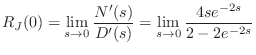
We already discovered a root at
 |
(C.166) |
and once again the limit is an indeterminate
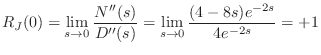 |
(C.167) |
Thus, two poles and zeros cancel at dc, and the dc reflectance is
Another method of showing this result is to form a Taylor series expansion
of the numerator and denominator:
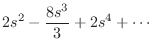 |
(C.168) | ||
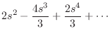 |
(C.169) |
Both series begin with the term
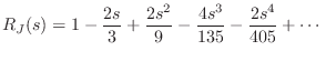 |
(C.170) |
which approaches
An alternative analysis of this issue is given by Benade in [37].
Next Section:
Finite-Difference Schemes
Previous Section:
The Digital Waveguide Oscillator