Excitation Examples
Localized Displacement Excitations
Whenever two adjacent components of

will initialize only
![]() , a solitary left-going pulse
of amplitude 1 at time
, a solitary left-going pulse
of amplitude 1 at time
![]() , as can be seen from Eq.
, as can be seen from Eq.![]() (E.11) by adding the leftmost columns
explicitly written for
(E.11) by adding the leftmost columns
explicitly written for
![]() . Similarly, the initialization
. Similarly, the initialization
gives rise to an isolated right-going pulse
![]() , corresponding
to the leftmost column of
, corresponding
to the leftmost column of
![]() plus the first column on the left not
explicitly written in Eq.
plus the first column on the left not
explicitly written in Eq.![]() (E.11). The superposition of these two
examples corresponds to a physical impulsive excitation at time 0 and
position
(E.11). The superposition of these two
examples corresponds to a physical impulsive excitation at time 0 and
position ![]() :
:
Thus, the impulse starts out with amplitude 2 at time 0 and position
In summary, we see that to excite a single sample of displacement
traveling in a single-direction, we must excite equally a pair of
adjacent colums in
![]() . This corresponds to equally weighted
excitation of K-variable pairs the form
. This corresponds to equally weighted
excitation of K-variable pairs the form
![]() .
.
Note that these examples involved only one of the two interleaved computational grids. Shifting over an odd number of spatial samples to the left or right would involve the other grid, as would shifting time forward or backward an odd number of samples.
Localized Velocity Excitations
Initial velocity excitations are straightforward in the DW paradigm,
but can be less intuitive in the FDTD domain. It is well known that
velocity in a displacement-wave DW simulation is determined by the
difference of the right- and left-going waves
[437]. Specifically, initial velocity waves ![]() can
be computed from from initial displacement waves
can
be computed from from initial displacement waves ![]() by spatially
differentiating
by spatially
differentiating ![]() to obtain traveling slope waves
to obtain traveling slope waves
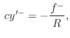
![]() , multiplying by minus the tension
, multiplying by minus the tension ![]() to obtain force
waves, and finally dividing by the wave impedance
to obtain force
waves, and finally dividing by the wave impedance
![]() to
obtain velocity waves:
to
obtain velocity waves:

where
We can see from Eq.![]() (E.11) that such asymmetry can be caused by
unequal weighting of
(E.11) that such asymmetry can be caused by
unequal weighting of ![]() and
and
![]() . For example, the
initialization
. For example, the
initialization
corresponds to an impulse velocity excitation at position
![]() . In this case, both interleaved grids are excited.
. In this case, both interleaved grids are excited.
More General Velocity Excitations
From Eq.![]() (E.11), it is clear that initializing any single K variable
(E.11), it is clear that initializing any single K variable
![]() corresponds to the initialization of an infinite number of W
variables
corresponds to the initialization of an infinite number of W
variables
![]() and
and
![]() . That is, a single K variable
. That is, a single K variable ![]() corresponds to only a single column of
corresponds to only a single column of
![]() for only one of the
interleaved grids. For example,
referring to Eq.
for only one of the
interleaved grids. For example,
referring to Eq.![]() (E.11),
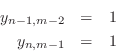
initializing the K variable
(E.11),
initializing the K variable
![]() to -1 at time
to -1 at time ![]() (with all other
(with all other ![]() intialized to 0)
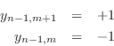
corresponds to the W-variable initialization
intialized to 0)
corresponds to the W-variable initialization
with all other W variables being initialized to zero.
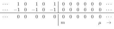
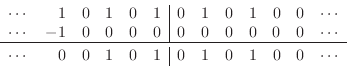
In view of earlier remarks, this corresponds to an impulsive velocity
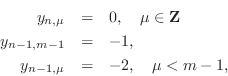
excitation on only one of the two subgrids. A schematic
depiction from ![]() to
to ![]() of the W variables at time
of the W variables at time ![]() is as
follows:
is as
follows:
 |
(E.14) |
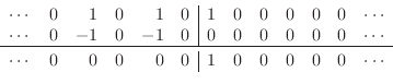
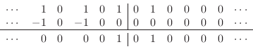
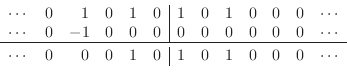
Below the solid line is the sum of the left- and right-going traveling-wave components, i.e., the corresponding K variables at time
 |
(E.15) |
 |
(E.16) |
 |
(E.17) |
 |
(E.18) |
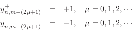
The sequence
Due to the independent interleaved subgrids in the FDTD algorithm, it is nearly always non-physical to excite only one of them, as the above example makes clear. It is analogous to illuminating only every other pixel in a digital image. However, joint excitation of both grids may be accomplished either by exciting adjacent spatial samples at the same time, or the same spatial sample at successive times instants.
In addition to the W components being non-local, they can demand a
larger dynamic range than the K variables. For example, if the entire
semi-infinite string for ![]() is initialized with velocity
is initialized with velocity ![]() ,
the initial displacement traveling-wave components look as follows:
,
the initial displacement traveling-wave components look as follows:
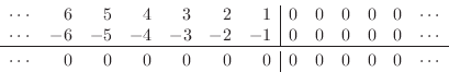 |
(E.19) |
and the variables evolve forward in time as follows:
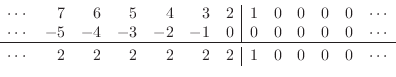 |
(E.20) |
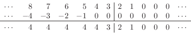 |
(E.21) |
 |
(E.22) |
Thus, the left semi-infinite string moves upward at a constant velocity of 2, while a ramp spreads out to the left and right of position
where ![]() denotes the set of all integers.
While the FDTD excitation is also not local, of course, it is
bounded for all
denotes the set of all integers.
While the FDTD excitation is also not local, of course, it is
bounded for all ![]() .
.
Since the traveling-wave components of initial velocity excitations are generally non-local in a displacement-based simulation, as illustrated in the preceding examples, it is often preferable to use velocity waves (or force waves) in the first place [447].
Another reason to prefer force or velocity waves is that displacement
inputs are inherently impulsive. To see why this is so, consider that
any physically correct driving input must effectively exert some
finite force on the string, and this force is free to change
arbitrarily over time. The ``equivalent circuit'' of the infinitely
long string at the driving point is a ``dashpot'' having real,
positive resistance
![]() . The applied force
. The applied force ![]() can be
divided by
can be
divided by ![]() to obtain the velocity
to obtain the velocity ![]() of the string driving
point, and this velocity is free to vary arbitrarily over time,
proportional to the applied force. However, this velocity must be
time-integrated to obtain a displacement
of the string driving
point, and this velocity is free to vary arbitrarily over time,
proportional to the applied force. However, this velocity must be
time-integrated to obtain a displacement ![]() . Therefore,
there can be no instantaneous displacement response to a finite
driving force. In other words, any instantaneous effect of an input
driving signal on an output displacement sample is non-physical except
in the case of a massless system. Infinite force is required to move
the string instantaneously. In sampled displacement simulations, we
must interpret displacement changes as resulting from time-integration
over a sampling period. As the sampling rate increases, any
physically meaningful displacement driving signal must converge to
zero.
. Therefore,
there can be no instantaneous displacement response to a finite
driving force. In other words, any instantaneous effect of an input
driving signal on an output displacement sample is non-physical except
in the case of a massless system. Infinite force is required to move
the string instantaneously. In sampled displacement simulations, we
must interpret displacement changes as resulting from time-integration
over a sampling period. As the sampling rate increases, any
physically meaningful displacement driving signal must converge to
zero.
Additive Inputs
Instead of initial conditions, ongoing input signals can be defined
analogously. For example, feeding an input signal ![]() into the FDTD
via
into the FDTD
via
corresponds to physically driving a single sample of string displacement at position
Interpretation of the Time-Domain KW Converter
As shown above, driving a single displacement sample ![]() in the
FDTD corresponds to driving a velocity input at position
in the
FDTD corresponds to driving a velocity input at position ![]() on two
alternating subgrids over time. Therefore, the filter
on two
alternating subgrids over time. Therefore, the filter
![]() acts as the filter
acts as the filter
![]() on either subgrid alone--a
first-order difference. Since displacement is being simulated, velocity
inputs must be numerically integrated. The first-order difference can
be seen as canceling this integration, thereby converting a velocity
input to a displacement input, as in Eq.
on either subgrid alone--a
first-order difference. Since displacement is being simulated, velocity
inputs must be numerically integrated. The first-order difference can
be seen as canceling this integration, thereby converting a velocity
input to a displacement input, as in Eq.![]() (E.23).
(E.23).
Next Section:
State Space Formulation
Previous Section:
State Transformations