The Clarinet Tonehole as a Two-Port Junction
![\includegraphics[scale=0.9]{eps/fFingerHoleKeefe}](http://www.dsprelated.com/josimages_new/pasp/img2398.png)
The clarinet tonehole model developed by Keefe [240] is
parametrized in terms of series and shunt resistance and reactance, as
shown in Fig. 9.43. The transmission
matrix description of this two-port is given by the product of the
transmission matrices for the series impedance ![]() , shunt
impedance
, shunt
impedance ![]() , and series impedance
, and series impedance ![]() , respectively:
, respectively:
![$\displaystyle \left[\begin{array}{c} P_1 \\ [2pt] U_1 \end{array}\right]$](http://www.dsprelated.com/josimages_new/pasp/img2401.png)
![$\displaystyle \left[\begin{array}{cc} 1 & R_a/2 \\ [2pt] 0 & 1 \end{array}\righ...
...1 \end{array}\right]
\left[\begin{array}{c} P_2 \\ [2pt] U_2 \end{array}\right]$](http://www.dsprelated.com/josimages_new/pasp/img2402.png)
![$\displaystyle \left[\begin{array}{cc} 1+\frac{R_a}{2R_s} & R_a[1+\frac{R_a}{4R_...
...} \end{array}\right]
\left[\begin{array}{c} P_2 \\ [2pt] U_2 \end{array}\right]$](http://www.dsprelated.com/josimages_new/pasp/img2403.png)
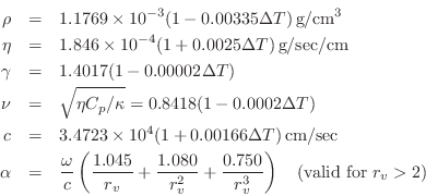
where all quantities are written in the frequency domain, and the impedance parameters are given by
| (open-hole shunt impedance) |
|||
| (closed-hole shunt impedance) |
(10.51) | ||
| (open-hole series impedance) |
|||
| (closed-hole series impedance) |
where
 |
|||
 |
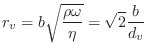
where
![$\displaystyle t_h = t_w + \frac{1}{8}\frac{b^2}{a}\left[1+0.172\left(\frac{b}{a}\right)^2\right]
$](http://www.dsprelated.com/josimages_new/pasp/img2426.png)
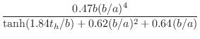
Note that the specific resistance of the open tonehole, ![]() , is the
only real impedance and therefore the only source of wave energy loss at
the tonehole. It is given by [240]
, is the
only real impedance and therefore the only source of wave energy loss at
the tonehole. It is given by [240]

![$\displaystyle \alpha = \frac{1}{2bc}\left[\,\sqrt{\frac{2\eta\omega}{\rho}}
+ (\gamma-1)\sqrt{\frac{2\kappa\omega}{\rho C_p}}\,\right]
$](http://www.dsprelated.com/josimages_new/pasp/img2433.png)
where
The open-hole effective length ![]() , assuming no pad above the hole,
is given in
[240] as
, assuming no pad above the hole,
is given in
[240] as
![$\displaystyle t_e = \frac{(1/k)\tan(kt) + b [1.40 - 0.58(b/a)^2]}{1 - 0.61 kb \tan(kt)}
$](http://www.dsprelated.com/josimages_new/pasp/img2445.png)
For implementation in a digital waveguide model, the lumped parameters above must be converted to scattering parameters. Such formulations of toneholes have appeared in the literature: Vesa Välimäki [509,502] developed tonehole models based on a ``three-port'' digital waveguide junction loaded by an inertance, as described in Fletcher and Rossing [143], and also extended his results to the case of interpolated digital waveguides. It should be noted in this context, however, that in the terminology of Appendix C, Välimäki's tonehole representation is a loaded 2-port junction rather than a three-port junction. (A load can be considered formally equivalent to a ``waveguide'' having wave impedance given by the load impedance.) Scavone and Smith [402] developed digital waveguide tonehole models based on the more rigorous ``symmetric T'' acoustic model of Keefe [240], using general purpose digital filter design techniques to obtain rational approximations to the ideal tonehole frequency response. A detailed treatment appears in Scavone's CCRMA Ph.D. thesis [406]. This section, adapted from [465], considers an exact translation of the Keefe tonehole model, obtaining two one-filter implementations: the ``shared reflectance'' and ``shared transmittance'' forms. These forms are shown to be stable without introducing an approximation which neglects the series inertance terms in the tonehole model.
By substituting
![]() in (9.53) to convert spatial
frequency to temporal frequency, and by substituting
in (9.53) to convert spatial
frequency to temporal frequency, and by substituting
| (10.52) | |||
 |
(10.53) |
for
        Clear["t*", "p*", "u*", "r*"]
        transmissionMatrix = {{t11, t12}, {t21, t22}};
        leftPort = {{p2p+p2m}, {(p2p-p2m)/r2}};
        rightPort = {{p1p+p1m}, {(p1p-p1m)/r1}};
        Format[t11, TeXForm] := "{T_{11}}"
        Format[p1p, TeXForm] := "{P_1^+}"
        ... (etc. for all variables) ...
        TeXForm[Simplify[Solve[leftPort ==
               transmissionMatrix . rightPort, {p1m, p2p}]]]
The above code produces the following formulas:
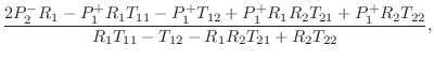
Substituting relevant values for Keefe's tonehole model, we obtain, in matrix notation,
![$\displaystyle \left[\begin{array}{c} P_1^{-} \\ [2pt] P_2^{+} \end{array}\right]$](http://www.dsprelated.com/josimages_new/pasp/img2459.png)
![$\displaystyle \left[\begin{array}{cc} S & T \\ [2pt] T & S \end{array}\right]
\left[\begin{array}{c} P_1^{+} \\ [2pt] P_2^{-} \end{array}\right]$](http://www.dsprelated.com/josimages_new/pasp/img2460.png)
![$\displaystyle \quad
\left[\begin{array}{cc} 4R_aR_s + R_a^2 - 4R_0^2 & 8R_0R_s ...
...rray}\right]
\left[\begin{array}{c} P_1^{+} \\ [2pt] P_2^{-} \end{array}\right]$](http://www.dsprelated.com/josimages_new/pasp/img2462.png)
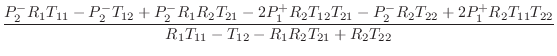
We thus obtain the scattering formulation depicted in Fig. 9.44, where
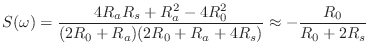
is the reflectance of the tonehole (the same from either direction), and
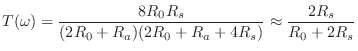
is the transmittance of the tonehole (also the same from either direction). The notation ``
![\includegraphics[scale=0.9]{eps/fFingerHoleScat}](http://www.dsprelated.com/josimages_new/pasp/img2465.png)
The approximate forms in (9.57) and (9.58) are obtained by neglecting
the negative series inertance ![]() which serves to adjust the effective
length of the bore, and which therefore can be implemented elsewhere in the
interpolated delay-line calculation as discussed further below. The open
and closed tonehole cases are obtained by substituting
which serves to adjust the effective
length of the bore, and which therefore can be implemented elsewhere in the
interpolated delay-line calculation as discussed further below. The open
and closed tonehole cases are obtained by substituting
![]() and
and
![]() , respectively, from (9.53).
, respectively, from (9.53).
In a manner analogous to converting the four-multiply Kelly-Lochbaum (KL)
scattering junction
[245]
into a one-multiply form (cf. (C.60) and
(C.62) on page ![]() ), we may pursue a ``one-filter'' form of the waveguide
tonehole model. However, the series inertance gives some initial trouble,
since
), we may pursue a ``one-filter'' form of the waveguide
tonehole model. However, the series inertance gives some initial trouble,
since
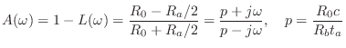
![$\displaystyle [1+S(\omega)] - T(\omega) = \frac{2R_a}{2R_0+ R_a} \isdef L(\omega)
$](http://www.dsprelated.com/josimages_new/pasp/img2469.png)
| (10.58) |
and, similarly,
| (10.59) |
The resulting tonehole implementation is shown in Fig. 9.45. We call this the ``shared reflectance'' form of the tonehole junction.
In the same way, an alternate form is obtained from the substitution
| (10.60) | |||
| (10.61) |
shown in Fig. 9.46.
![\includegraphics[scale=0.9]{eps/fFingerHoleOneMul}](http://www.dsprelated.com/josimages_new/pasp/img2485.png)
![\includegraphics[scale=0.9]{eps/fFingerHoleOneMulAlt}](http://www.dsprelated.com/josimages_new/pasp/img2486.png)
![\includegraphics[scale=0.9]{eps/fFingerHoleOneMulCommuted}](http://www.dsprelated.com/josimages_new/pasp/img2487.png) |
![\includegraphics[width=\twidth]{eps/fFingerHoleOneMulAltCommuted}](http://www.dsprelated.com/josimages_new/pasp/img2488.png)
Since
![]() , it can be neglected to first order, and
, it can be neglected to first order, and
![]() , reducing both of the above forms to an approximate
``one-filter'' tonehole implementation.
, reducing both of the above forms to an approximate
``one-filter'' tonehole implementation.
Since
![]() is a pure negative reactance, we have
is a pure negative reactance, we have
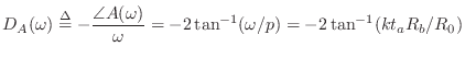
In this form, it is clear that
We now see precisely how the negative series inertance ![]() provides a
negative, frequency-dependent, length correction for the bore. From
(9.63),
the phase delay of
provides a
negative, frequency-dependent, length correction for the bore. From
(9.63),
the phase delay of ![]() can be computed as
can be computed as
In practice, it is common to combine all delay corrections into a single ``tuning allpass filter'' for the whole bore [428,207]. Whenever the desired allpass delay goes negative, we simply add a sample of delay to the desired allpass phase-delay and subtract it from the nearest delay. In other words, negative delays have to be ``pulled out'' of the allpass and used to shorten an adjacent interpolated delay line. Such delay lines are normally available in practical modeling situations.
Next Section:
Tonehole Filter Design
Previous Section:
Clarinet Synthesis Implementation Details