Adaptors for Wave Digital Elements
An adaptor is an ![]() -port memoryless interface which
interconnects wave digital elements. Since each element's ``port'' is
a connection to an infinitesimal waveguide section at some real wave
impedance
-port memoryless interface which
interconnects wave digital elements. Since each element's ``port'' is
a connection to an infinitesimal waveguide section at some real wave
impedance ![]() , and since the input/output signals are wave
variables (traveling-waves within the waveguide), the adaptor must
implement signal scattering appropriate for the connection of
such waveguides. In other words, an
, and since the input/output signals are wave
variables (traveling-waves within the waveguide), the adaptor must
implement signal scattering appropriate for the connection of
such waveguides. In other words, an ![]() -port adaptor in a wave
digital filter performs exactly the same computation as an
-port adaptor in a wave
digital filter performs exactly the same computation as an ![]() -port
scattering junction in a digital waveguide network.F.2
-port
scattering junction in a digital waveguide network.F.2
This section first addresses the simpler two-port case, followed by a
derivation of the general ![]() -port adaptor, for both parallel and
series connections of wave digital elements.
-port adaptor, for both parallel and
series connections of wave digital elements.
As discussed in §7.2, a physical connection of two or more ports can either be in parallel (forces are equal and the velocities sum to zero) or in series (velocities equal and forces sum to zero). Combinations of parallel and series connections are also of course possible.
Two-Port Parallel Adaptor for Force Waves
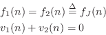
Figure F.5a illustrates a generic parallel two-port connection in terms of forces and velocities.
![\includegraphics[width=\twidth]{eps/lAdaptorParallel}](http://www.dsprelated.com/josimages_new/pasp/img4823.png) |
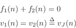
As discussed in §7.2, a parallel connection is characterized by a common force and velocities which sum to zero:
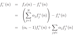
Following the same derivation leading to Eq.![]() (F.2), and defining
(F.2), and defining
![]() for notational convenience, we obtain
for notational convenience, we obtain
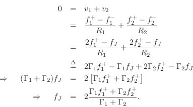
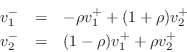
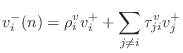
The outgoing wave variables are given by
Defining the reflection coefficient as

as diagrammed in Fig.F.5b. This can be called the Kelly-Lochbaum implementation of the two-port force-wave adaptor.
Now that we have a proper scattering interface between two reference
impedances, we may connect two wave digital elements together, setting
![]() to the port impedance of element 1, and
to the port impedance of element 1, and ![]() to the port
impedance of element 2. An example is shown in Fig.F.35.
to the port
impedance of element 2. An example is shown in Fig.F.35.
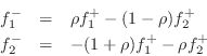
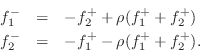
The Kelly-Lochbaum adaptor in Fig.F.5b evidently requires four multiplies and two additions. Note that we can factor out the reflection coefficient in each equation to obtain
which requires only one multiplication and three additions. This can be called the one-multiply form. The one-multiply form is most efficient in custom VLSI. The Kelly-Lochbaum form, on the other hand, may be more efficient in software, and slightly faster (by one addition) in parallel hardware.
Compatible Port Connections
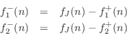
Note carefully that to connect a wave digital element to port
![]() of the adaptor, we route the signal
of the adaptor, we route the signal
![]() coming out of the
element to become
coming out of the
element to become
![]() on the adaptor port, and the signal
on the adaptor port, and the signal
![]() coming out of port
coming out of port ![]() of the adaptor goes into the element
as
of the adaptor goes into the element
as
![]() . Such a connection is said to be a
compatible port connection. In other words, the connections
must be made such that the arrows go in the same direction in the wave
flow diagram.
. Such a connection is said to be a
compatible port connection. In other words, the connections
must be made such that the arrows go in the same direction in the wave
flow diagram.
General Parallel Adaptor for Force Waves
In the more general case of ![]() wave digital element ports being
connected in parallel, we have the physical constraints
wave digital element ports being
connected in parallel, we have the physical constraints
| (F.14) | |||
| (F.15) |
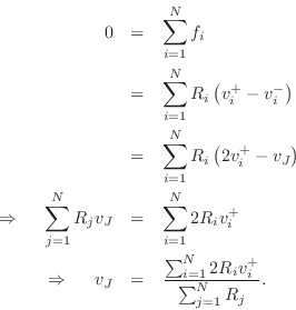
The derivation for the two-port case extends to the


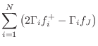


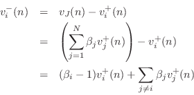
The outgoing wave variables are given by
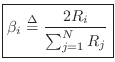
Alpha Parameters
It is customary in the wave digital filter literature to define the alpha parameters as
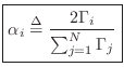
where

We see that

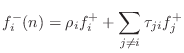
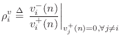
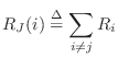
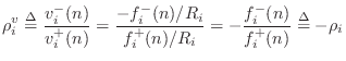
Reflection Coefficient, Parallel Case
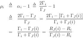
The reflection coefficient seen at port ![]() is defined as
is defined as
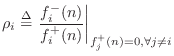
In other words, the reflection coefficient specifies what portion of the incoming wave
where
Equating like terms with Eq.![]() (F.21), we obtain
(F.21), we obtain
Thus, the
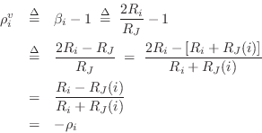
Physical Derivation of Reflection Coefficient
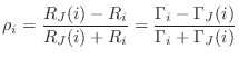
Physically, the reflection coefficient seen at port ![]() is due to an
impedance step from
is due to an
impedance step from ![]() , that of the port interface, to a new
impedance consisting of the parallel combination of all other
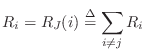
port impedances meeting at the junction. Let
, that of the port interface, to a new
impedance consisting of the parallel combination of all other
port impedances meeting at the junction. Let
denote this parallel combination, in admittance form. Then we must have
Let's check this ``physical'' derivation against the formal definition
Eq.![]() (F.20) leading to
(F.20) leading to
![]() in Eq.
in Eq.![]() (F.22).
Toward this goal, let
(F.22).
Toward this goal, let

and the result is verified.
Reflection Free Port
It is useful in practice, such as when connecting two adaptors
together, to make one port reflection free. A
reflection-free port is defined to have a zero reflection coefficient. For port
![]() of a parallel adaptor to be reflection free, we must have, from
Eq.
of a parallel adaptor to be reflection free, we must have, from
Eq.![]() (F.25),
(F.25),
Connecting two adaptors at a reflection-free port prevents the formation of a delay-free loop which would otherwise occur [136]. As a result, multi-port junctions can be joined without having to insert unit elements (see §F.1.7) to avoid creating delay-free loops. Only one of the two ports participating in the connection needs to be reflection free.
We can always make a reflection-free port at the connection of two adaptors because the ports used for this connection (one on each adaptor) were created only for purposes of this connection. They can be set to any impedance, and only one of them needs to be reflection free.
To interconnect three adaptors, labeled ![]() ,
, ![]() , and
, and ![]() , we may
proceed as follows: Let
, we may
proceed as follows: Let ![]() be augmented with two unconstrained
ports, having impedances
be augmented with two unconstrained
ports, having impedances ![]() and
and ![]() . Add a reflection-free
port to
. Add a reflection-free
port to ![]() , and suppose its impedance has to be
, and suppose its impedance has to be ![]() . Add a
reflection-free port to
. Add a
reflection-free port to ![]() , and suppose its impedance has to be
, and suppose its impedance has to be
![]() . Now set
. Now set ![]() and connect
and connect ![]() to
to ![]() via the
corresponding ports. Similarly, set
via the
corresponding ports. Similarly, set ![]() and connect
and connect ![]() to
to ![]() accordingly. This adaptor-connection protocol clearly extends to any
number of adaptors.
accordingly. This adaptor-connection protocol clearly extends to any
number of adaptors.
Two-Port Series Adaptor for Force Waves
Figure F.6a illustrates a generic two-port description of the series adaptor.
![\includegraphics[width=\twidth]{eps/lAdaptorSeries}](http://www.dsprelated.com/josimages_new/pasp/img4871.png) |
As discussed in §7.2, a series connection is characterized by a common velocity and forces which sum to zero at the junction:
The derivation can proceed exactly as for the parallel junction in
§F.2.1, but with force and velocity interchanged, i.e.,
![]() , and with impedance and admittance interchanged,
i.e.,
, and with impedance and admittance interchanged,
i.e.,
![]() . In this way, we may take the
dual of Eq.
. In this way, we may take the
dual of Eq.![]() (F.14) to get
(F.14) to get
diagrammed in Fig.F.7. Converting back to force wave
variables via
![]() and
and
![]() , and noting
that
, and noting
that
![]() , we obtain, finally,
, we obtain, finally,
as diagrammed in Fig.F.6b. The one-multiply form is now
![\includegraphics[scale=0.9]{eps/lscat_vel_series_renum}](http://www.dsprelated.com/josimages_new/pasp/img4881.png)
General Series Adaptor for Force Waves
In the more general case of ![]() ports being connected in
series, we have the physical constraints
ports being connected in
series, we have the physical constraints

The derivation is the dual of that in the parallel case (cf.
Eq.![]() (F.16)), i.e., force and velocity are interchanged, and impedance
and admittance are interchanged:
(F.16)), i.e., force and velocity are interchanged, and impedance
and admittance are interchanged:
The outgoing wave variables are given by
Beta Parameters
It is customary in the wave digital filter literature to define the beta parameters as
where

However, we normally employ a mixture of parallel and series adaptors,
while keeping a force-wave simulation. Since
![]() , we obtain, after a small amount of algebra, the following
recipe for the series force-wave adaptor:
, we obtain, after a small amount of algebra, the following
recipe for the series force-wave adaptor:

We see that we have

Reflection Coefficient, Series Case
The velocity reflection coefficient seen at port
![]() is defined as
is defined as
Representing the outgoing velocity wave
where
Equating like terms with Eq.![]() (F.32) gives
(F.32) gives
Thus, the
Physical Derivation of Series Reflection Coefficient
Physically, the force-wave reflection coefficient seen at port
![]() of a series adaptor is due to an impedance step from
of a series adaptor is due to an impedance step from ![]() , that
of the port interface, to a new impedance consisting of the series
combination of all other port impedances meeting at the
junction. Let
, that
of the port interface, to a new impedance consisting of the series
combination of all other port impedances meeting at the
junction. Let
denote this series combination. Then we must have, as in Eq.
 |
(F.36) |
Let's check this ``physical'' derivation against the formal definition
Eq.![]() (F.31) leading to
(F.31) leading to
![]() in Eq.
in Eq.![]() (F.33).
Define the total junction impedance as
(F.33).
Define the total junction impedance as

Since
Series Reflection Free Port
For port ![]() to be reflection free in a series adaptor, we require
to be reflection free in a series adaptor, we require
That is, the port's impedance must equal the series combination of the other port impedances at the junction. This result can be compared with that for the parallel junction in §F.2.2.
The series adaptor has now been derived in a way which emphasizes its duality with respect to the parallel adaptor.
Next Section:
Wave Digital Modeling Examples
Previous Section:
Wave Digital Elements