Elementary Filter Sections
This section gives condensed analysis summaries of the four most
elementary digital filters: the one-zero, one-pole, two-pole, and
two-zero filters. Despite their relative simplicity, they are quite
valuable to master in practice. In particular, recall from
Chapter 9 that every causal, finite-order, LTI filter (any
difference equation of the form
Eq.![]() (5.1)) may be factored into a series and/or parallel
combinationof such sections. Implementing high-order filters as parallel and/or
series combinations of low-order sections offers several advantages,
such as numerical robustness and easier/safer control in real time.
(5.1)) may be factored into a series and/or parallel
combinationof such sections. Implementing high-order filters as parallel and/or
series combinations of low-order sections offers several advantages,
such as numerical robustness and easier/safer control in real time.
One-Zero
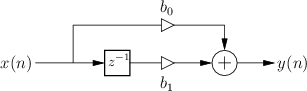
Figure B.1 gives the signal flow graph for the general one-zero filter. The frequency response for the one-zero filter may be found by the following steps:

By factoring out
![]() from the frequency response, to
balance the exponents of
from the frequency response, to
balance the exponents of ![]() , we can get this closer to polar form as
follows:
, we can get this closer to polar form as
follows:
 |
We now apply the general equations given in
Chapter 7 for filter gain ![]() and filter phase
and filter phase
![]() as a function of frequency:
as a function of frequency:
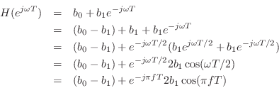
![\begin{eqnarray*}
H(e^{j\omega T}) &=& b_0 + b_1e^{-j\omega T}\\
&=& b_0 + b_1...
...left[\frac{-b_1 \sin(\omega T)}{b_0 + b_1 \cos(\omega T)}\right]
\end{eqnarray*}](http://www.dsprelated.com/josimages_new/filters/img1343.png)
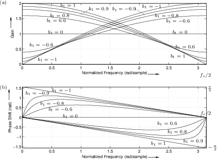
A plot of ![]() and
and
![]() for
for ![]() and various
real values of
and various
real values of ![]() , is given in Fig.B.2. The filter has a zero
at
, is given in Fig.B.2. The filter has a zero
at
![]() in the
in the ![]() plane, which is always on the
real axis. When a point on the unit circle comes close to the zero of
the transfer function the filter gain at that frequency is
low. Notice that one real zero can basically make either a highpass
(
plane, which is always on the
real axis. When a point on the unit circle comes close to the zero of
the transfer function the filter gain at that frequency is
low. Notice that one real zero can basically make either a highpass
(
![]() ) or a lowpass filter (
) or a lowpass filter (
![]() ). For the phase
response calculation using the graphical method, it is necessary to
include the pole at
). For the phase
response calculation using the graphical method, it is necessary to
include the pole at ![]() .
.
One-Pole
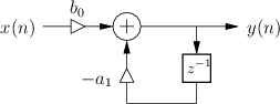
Fig.B.3 gives the signal flow graph for the general one-pole filter. The road to the frequency response goes as follows:
 |
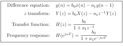
The one-pole filter has a transfer function (hence frequency response) which is the reciprocal of that of a one-zero. The analysis is thus quite analogous. The frequency response in polar form is given by
![\begin{eqnarray*}
G(\omega) &=& \frac{\vert b_0\vert}{\sqrt{[1 + a_1 \cos(\omega...
... + a_1 \cos(\omega T)}\right], & b_0<0 \\
\end{array} \right..
\end{eqnarray*}](http://www.dsprelated.com/josimages_new/filters/img1351.png)
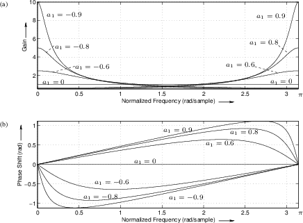
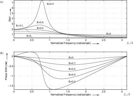
A plot of the frequency response in polar form for ![]() and
various values of
and
various values of ![]() is given in Fig.B.4.
is given in Fig.B.4.
The filter has a pole at ![]() , in the
, in the ![]() plane (and a zero at
plane (and a zero at ![]() = 0). Notice that the one-pole exhibits
either a lowpass or a highpass frequency response, like the
one-zero. The lowpass character occurs when the pole is near the point
= 0). Notice that the one-pole exhibits
either a lowpass or a highpass frequency response, like the
one-zero. The lowpass character occurs when the pole is near the point
![]() (dc), which happens when
(dc), which happens when ![]() approaches
approaches ![]() . Conversely,
the highpass nature occurs when
. Conversely,
the highpass nature occurs when ![]() is positive.
is positive.
The one-pole filter section can achieve much more drastic differences
between the gain at high frequencies and the gain at low frequencies
than can the one-zero filter. This difference is achieved in the
one-pole by gain boost in the passband rather than
attenuation in the stopband; thus it is usually desirable when
using a one-pole filter to set ![]() to a small value, such as
to a small value, such as
![]() , so that the peak gain is 1 or so. When the peak gain is 1,
the filter is unlikely to overflow.B.1
, so that the peak gain is 1 or so. When the peak gain is 1,
the filter is unlikely to overflow.B.1
Finally, note that the one-pole filter is stable if and only if
![]() .
.
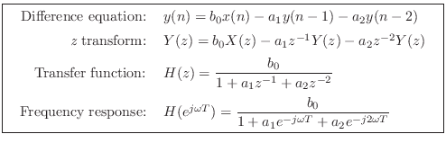
Two-Pole
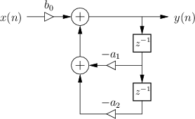
The signal flow graph for the general two-pole filter is given in Fig.B.5. We proceed as usual with the general analysis steps to obtain the following:
The numerator of ![]() is a constant, so there are no zeros other
than two at the origin of the
is a constant, so there are no zeros other
than two at the origin of the ![]() plane.
plane.
The coefficients ![]() and
and ![]() are called the denominator
coefficients, and they determine the two poles of
are called the denominator
coefficients, and they determine the two poles of ![]() .
Using the quadratic formula, the poles are found to be located at
.
Using the quadratic formula, the poles are found to be located at
When both poles are real, the two-pole can be analyzed simply as a cascade of two one-pole sections, as in the previous section. That is, one can multiply pointwise two magnitude plots such as Fig.B.4a, and add pointwise two phase plots such as Fig.B.4b.
When the poles are complex, they can be written as
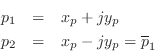
since they must form a complex-conjugate pair when ![]() and
and ![]() are real.
We may express them in polar form
as
are real.
We may express them in polar form
as
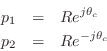
where
![]() is the pole radius, or distance from the origin in the
is the pole radius, or distance from the origin in the
![]() -plane. As discussed in Chapter 8, we must have
-plane. As discussed in Chapter 8, we must have ![]() for
stability of the two-pole filter. The angles
for
stability of the two-pole filter. The angles
![]() are the
poles' respective angles in the
are the
poles' respective angles in the ![]() plane. The pole angle
plane. The pole angle
![]() corresponds to the pole frequency
corresponds to the pole frequency ![]() via the
relation
via the
relation
If ![]() is sufficiently large (but less than 1 for stability), the
filter exhibits a resonanceB.2 at
radian frequency
is sufficiently large (but less than 1 for stability), the
filter exhibits a resonanceB.2 at
radian frequency
![]() . We may call
. We may call
![]() or
or ![]() the center frequency of the
resonator. Note, however, that the resonance frequency is not usually
the precise frequency of peak-gain in a two-pole resonator (see
Fig.B.9 on page
the center frequency of the
resonator. Note, however, that the resonance frequency is not usually
the precise frequency of peak-gain in a two-pole resonator (see
Fig.B.9 on page ![]() ).
The peak of the amplitude response is usually a little different
because each pole sits on the other's ``skirt,'' which is slanted.
(See §B.1.5 and §B.6 for an elaboration of this point.)
).
The peak of the amplitude response is usually a little different
because each pole sits on the other's ``skirt,'' which is slanted.
(See §B.1.5 and §B.6 for an elaboration of this point.)
Using polar form for the (complex) poles, the two-pole transfer
function can be expressed as
Comparing this to the transfer function derived from the difference equation, we may identify
The difference equation can thus be rewritten as
Note that coefficient ![]() depends only on the pole radius R (which
determines damping) and is independent of the resonance frequency,
while
depends only on the pole radius R (which
determines damping) and is independent of the resonance frequency,
while ![]() is a function of both. As a result, we may retune
the resonance frequency of the two-pole filter section by modifying
is a function of both. As a result, we may retune
the resonance frequency of the two-pole filter section by modifying
![]() only.
only.
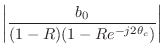
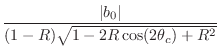
The gain at the resonant frequency
![]() , is found by
substituting
, is found by
substituting
![]() into
Eq.
into
Eq.![]() (B.1) to get
(B.1) to get
See §B.6 for details on how the resonance
gain (and peak gain) can be normalized as the tuning of ![]() is
varied in real time.
is
varied in real time.
Since the radius of both poles is ![]() , we must have
, we must have ![]() for filter
stability (§8.4). The
closer
for filter
stability (§8.4). The
closer ![]() is to 1, the higher the gain at the resonant frequency
is to 1, the higher the gain at the resonant frequency
![]() . If
. If ![]() , the filter degenerates to the form
, the filter degenerates to the form
![]() , which is a nothing but a scale factor. We can say that
when the two poles move to the origin of the
, which is a nothing but a scale factor. We can say that
when the two poles move to the origin of the ![]() plane, they are
canceled by the two zeros there.
plane, they are
canceled by the two zeros there.
Resonator Bandwidth in Terms of Pole Radius
The magnitude ![]() of a complex pole determines the
damping or bandwidth of the resonator. (Damping may be
defined as the reciprocal of the bandwidth.)
of a complex pole determines the
damping or bandwidth of the resonator. (Damping may be
defined as the reciprocal of the bandwidth.)
As derived in §8.5, when ![]() is close to 1, a reasonable
definition of 3dB-bandwidth
is close to 1, a reasonable
definition of 3dB-bandwidth ![]() is provided by
is provided by

where
Figure B.6 shows a family of frequency responses for the
two-pole resonator obtained by setting ![]() and varying
and varying ![]() . The
value of
. The
value of ![]() in all cases is
in all cases is ![]() , corresponding to
, corresponding to
![]() . The analytic expressions for amplitude and phase response are
. The analytic expressions for amplitude and phase response are
![\begin{eqnarray*}
G(\omega)\! &=&
\!\frac{b_0}{\sqrt{[1 + a_1 \cos(\omega T) + a...
... + a_1 \cos(\omega T) + a_2 \cos(2\omega T)}\right]\qquad(b_0>0)
\end{eqnarray*}](http://www.dsprelated.com/josimages_new/filters/img1385.png)
where
![]() and
and ![]() .
.
 |
Two-Zero
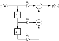
The signal flow graph for the general two-zero filter is given in Fig.B.7, and the derivation of frequency response is as follows:
![\fbox{
\begin{tabular}{rl}
Difference equation: & $y(n) = b_0 x(n) + b_1 x(n-1) ...
...+ b_1 \cos(\omega T) + b_2 \cos(2\omega T)}\right]$
\end{tabular}\vspace{10pt}
}](http://www.dsprelated.com/josimages_new/filters/img1389.png)
As discussed in §5.1,
the parameters ![]() and
and ![]() are called the numerator
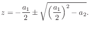
coefficients, and they determine the two zeros. Using the
quadratic formula for finding the roots of a second-order polynomial,
we find that the zeros are located at
are called the numerator
coefficients, and they determine the two zeros. Using the
quadratic formula for finding the roots of a second-order polynomial,
we find that the zeros are located at

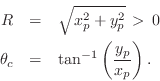
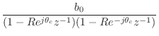
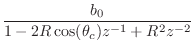
Forming a general two-zero transfer function in factored form gives
![\begin{eqnarray*}
H(z) &=& b_0 (1 - Re^{j\theta_c} z^{-1}) (1 - Re^{-j\theta_c} z^{-1})\\
&=& b_0 [1 - 2R\cos(\theta_c) z^{-1}+ R^2 z^{-2}]
\end{eqnarray*}](http://www.dsprelated.com/josimages_new/filters/img1397.png)
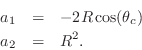
from which we identify
![]() and
and
![]() , so that
, so that
The approximate relation between bandwidth and ![]() given in
Eq.
given in
Eq.![]() (B.5) for the two-pole resonator now applies to the notch
width in the two-zero filter.
(B.5) for the two-pole resonator now applies to the notch
width in the two-zero filter.
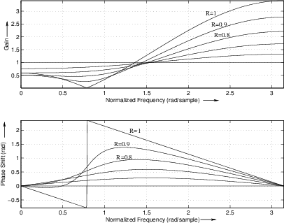
Figure B.8 gives some two-zero frequency responses obtained by
setting ![]() to 1 and varying
to 1 and varying ![]() . The value of
. The value of ![]() , is again
, is again
![]() . Note that the response is exactly analogous to the two-pole
resonator with notches replacing the resonant peaks. Since the plots
are on a linear magnitude scale, the two-zero amplitude response
appears as the reciprocal of a two-pole response. On a dB scale, the
two-zero response is an upside-down two-pole response.
. Note that the response is exactly analogous to the two-pole
resonator with notches replacing the resonant peaks. Since the plots
are on a linear magnitude scale, the two-zero amplitude response
appears as the reciprocal of a two-pole response. On a dB scale, the
two-zero response is an upside-down two-pole response.
 |
Complex Resonator
Normally when we need a resonator, we think immediately of the two-pole resonator. However, there is also a complex one-pole resonator having the transfer function
where
Since the impulse response is the inverse z transform of the
transfer function, we can write down the impulse response of the
complex one-pole resonator by recognizing Eq.![]() (B.6) as the
closed-form sum of an infinite geometric series, yielding
(B.6) as the
closed-form sum of an infinite geometric series, yielding
![$\displaystyle u(n) \isdef \left\{\begin{array}{ll}
1, & n\geq 0 \\ [5pt]
0, & n<0 \\
\end{array}\right.
$](http://www.dsprelated.com/josimages_new/filters/img1406.png)
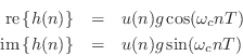
These may be called phase-quadrature sinusoids, since their phases differ by 90 degrees. The phase quadrature relationship for two sinusoids means that they can be regarded as the real and imaginary parts of a complex sinusoid.
By allowing ![]() to be complex,
to be complex,
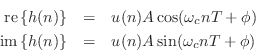
The frequency response of the complex one-pole resonator differs from
that of the two-pole real resonator in that the resonance
occurs only for one positive or negative frequency ![]() , but not
both. As a result, the resonance frequency
, but not
both. As a result, the resonance frequency ![]() is also the
frequency where the peak-gain occurs; this is only true in
general for the complex one-pole resonator. In particular, the peak
gain of a real two-pole filter does not occur exactly at resonance, except
when
is also the
frequency where the peak-gain occurs; this is only true in
general for the complex one-pole resonator. In particular, the peak
gain of a real two-pole filter does not occur exactly at resonance, except
when
![]() ,
, ![]() , or
, or ![]() . See
§B.6 for more on peak-gain versus resonance-gain (and how to
normalize them in practice).
. See
§B.6 for more on peak-gain versus resonance-gain (and how to
normalize them in practice).
Two-Pole Partial Fraction Expansion
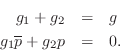
Note that every real two-pole resonator can be broken up into a sum of two complex one-pole resonators:
where
![\includegraphics[width=\twidth ]{eps/tppfe}](http://www.dsprelated.com/josimages_new/filters/img1419.png) |
To show Eq.![]() (B.7) is always true, let's solve in general for
(B.7) is always true, let's solve in general for ![]() and
and ![]() given
given ![]() and
and ![]() . Recombining the right-hand side
over a common denominator and equating numerators gives
. Recombining the right-hand side
over a common denominator and equating numerators gives
The solution is easily found to be
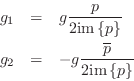
where we have assumed
im![]() , as necessary to have a
resonator in the first place.
, as necessary to have a
resonator in the first place.
Breaking up the two-pole real resonator into a parallel sum of two complex one-pole resonators is a simple example of a partial fraction expansion (PFE) (discussed more fully in §6.8).
Note that the inverse z transform of a sum of one-pole transfer
functions can be easily written down by inspection. In particular,
the impulse response of the PFE of the two-pole resonator (see
Eq.![]() (B.7)) is clearly
(B.7)) is clearly
The BiQuad Section
The term ``biquad'' is short for ``bi-quadratic'', and is a common name for a two-pole, two-zero digital filter. The transfer function of the biquad can be defined as
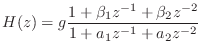
where
As derived in §B.1.3, for real second-order polynomials having
complex roots, it is often convenient to express the polynomial
coefficients in terms of the radius ![]() and angle
and angle ![]() of the
positive-frequency pole. For example, denoting the denominator
polynomial by
of the
positive-frequency pole. For example, denoting the denominator
polynomial by
![]() , we have
, we have
As discussed on page ![]() , a common setting for the zeros when
making a resonator is to place one at
, a common setting for the zeros when
making a resonator is to place one at ![]() (dc) and the other at
(dc) and the other at
![]() (half the sampling rate), i.e.,
(half the sampling rate), i.e., ![]() and
and
![]() in
Eq.
in
Eq.![]() (B.8) above
(B.8) above
![]() .
This zero placement normalizes the peak gain of the resonator if it is
swept using the
.
This zero placement normalizes the peak gain of the resonator if it is
swept using the ![]() parameter.
parameter.
Using the shift theorem for z transforms, the difference equation for the biquad can be written by inspection of the transfer function as
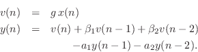
where ![]() denotes the input signal sample at time
denotes the input signal sample at time ![]() , and
, and ![]() is the output signal. This is the form that is typically implemented
in software. It is essentially the direct-form I implementation. (To obtain the official
direct-form I structure, the overall gain
is the output signal. This is the form that is typically implemented
in software. It is essentially the direct-form I implementation. (To obtain the official
direct-form I structure, the overall gain ![]() must be not be pulled
out separately, resulting in feedforward coefficients
must be not be pulled
out separately, resulting in feedforward coefficients
![]() instead. See Chapter 9 for more about
filter implementation forms.)
instead. See Chapter 9 for more about
filter implementation forms.)
Biquad Software Implementations
In matlab, an efficient biquad section is implemented by calling
outputsignal = filter(B,A,inputsignal);
where
![\begin{eqnarray*}
\texttt{B} &=& [g, g\beta_1, g\beta_2],\\
\texttt{A} &=& [1, a_1, a_2].
\end{eqnarray*}](http://www.dsprelated.com/josimages_new/filters/img1436.png)
A complete C++ class implementing a biquad filter section is included in the free, open-source Synthesis Tool Kit (STK) [15]. (See the BiQuad STK class.)
Figure B.10 lists an example biquad implementation in the C programming language.
typedef double *pp; // pointer to array of length NTICK typedef word double; // signal and coefficient data type typedef struct _biquadVars { pp output; pp input; word s2; word s1; word gain; word a2; word a1; word b2; word b1; } biquadVars; void biquad(biquadVars *a) { int i; dbl A; word s0; for (i=0; i<NTICK; i++) { A = a->gain * a->input[i]; A -= a->a1 * a->s1; A -= a->a2 * a->s2; s0 = A; A += a->b1 * a->s1; a->output[i] = a->b2 * a->s2 + A; a->s2 = a->s1; a->s1 = s0; } } |
Next Section:
Allpass Filter Sections
Previous Section:
A Sum of Sinusoids at the Same Frequency is Another Sinusoid at that Frequency